Fractal geometry can be used to create CAD models of complex shapes observed in the living organisms (cell, tissue, lung, blood vassals, brain structure, and alike) and in the natural world (tree, leaf, flower, landscape, coastline, cloud), as well. If one considers making a physical model of a fractal-geometry-generated CAD model, it is important to perform some topological transformations (e.g., concave/convex hull generation) for making the CAD model meaningful to the manufacturing devices. As a contribution in this area, this study describes a simple but effective procedure that can be used to generate concave hulls for fractal shapes generated by a random walk called Iterated Function System (IFS). One of the constituents of the proposed procedure is an in silico DNA-Based Computing. To demonstrate how the proposed concave hull generating procedure works, a case study has been performed, and using the information of the concave hull generated, a physical model of the fractal has been produced with the aid of additive manufacturing (3D printer).
fractals, concave/convex hull, DNA-based computing, additive manufacturing
Fractal geometry [1-3] can be used to create CAD models of complex shapes observed in the living organisms (cell, tissue, lung, blood vassals, brain structure, and alike) and in the natural world (tree, leaf, flower, landscape, coastline, cloud). If one considers making a physical model of a fractal-geometry-generated CAD model, it is important to perform some topological transformations for making the CAD model meaningful to the manufacturing devices. In doing so, creating concave/convex hulls [4-16] is a must. The concept of concave/convex hull is schematically illustrated in Figure 1. The shape used in Figure 1a is a point-cloud that models the shape of a fern-leaf created by a special random walk called Iterative Function System (IFS) [17,18]. The convex hull underlying the fern-leaf is shown in Figure 1b, which is the smallest perimeter fence enclosing the point-cloud. Some concave hulls (back and red boundaries) underlying the fern-leaf are shown in Figure 1c, which are the boundary fences encompassing the point-cloud as closely as possible. In case of concave hulls, internal and external boundary fences can be considered. For the case shown in Figure 1, the outer and internal concave hulls are shown by the black and red boundary fences, as seen from Figure 1c, respectively. Compared to the convex hull, concave hulls are more effective in preserving the shape information (compare the boundary fences shown in Figure 1b and 1c.
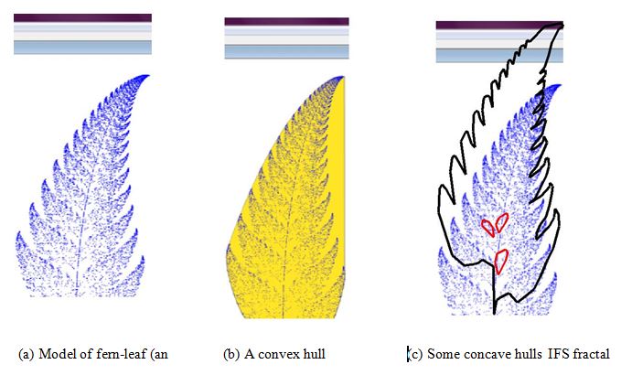
Figure 1. Concept of concave/convex hull
As mentioned before, if one considers making a physical model of a fractal shape from its CAD model (in the case of IFS fractals, the CAD model takes the form of a point-cloud), it is important to create a concave/convex hull first. The reason is that the concave/convex hull helps create other data (e.g., tool-paths [12,13] and STL data [19]) necessary for creating a physical model either by using subtractive manufacturing or by using additive manufacturing [12,13,16]. In certain cases, the remodeling of the fractal-geometry-generated CAD model is necessary for the sake of physical model building process [12,13,16,20]. Therefore, creating concave/convex hulls for the fractal-geometry-generated CAD model has been an active research topic. A series of systematic transformations is needed to make the information of the CAD model meaningful for the concave/convex hull generation procedure. Nevertheless, most of the procedures developed so far for generating concave/convex hull are computationally heavy. This article deals with this issue by proposing a new concave hull generating procedure, where the primary shape information is IFS-generated point-cloud (i.e., a fractal). The focus is on generating the outer concave hull, not the inner ones. One of the important constituents of the proposed procedure is a transformation that employs an in silico DNA-Based Computing (DBC) [21-24]. Thus, the remainder of this article is organized as follows. Section 2 describes the DBC employed in this article. Section 3 describes the proposed DBC driven outer concave hull generation procedure. Section 4 describes a case study showing the effectiveness of the proposed procedure. Section 5 provides the concluding remarks of this study.
A nature inspired computing methodology called DBC has been developed that takes the inspirations from the central dogma [25] of molecular biology. Central dogma of molecular biology simply means that once the sequential information of DNA/RNA has passed into protein (a sequence of amino acids) it cannot get out again [25]. A comprehensive description of the central dogma based DBC can be found in [21,22]. The remainder of this section briefly describes the DBC employed in this article for generating a concave hull.
Figure 2 schematically describes the form of DBC used in this article. In general, the DBC first maps a given binary array into DNA array. Finally, it maps the generated DNA array to a protein array (i.e., to a sequence of amino acids). The binary array must be a piece of information underlying the given problem (the point-cloud of the fractal shape created by a certain IFS). The protein array must help solve the given problem (in this case the concave hull creation problem).
As it is observed in Figure 2, DBC first maps the given binary array ∀bij ∈ {0,1} to an DNA array, ∀DNAij ∈ {A, C, G, T}. In doing so, two consecutive elements (bijbi+1j or bijbij+1 = 00, 01, 10, or 11) are mapped into one of the elements taken from {A, C, G, T}.
This process underlies four different types of reading-frame: continuous/discrete raw-/column-wise reading-frames. The case shown in Figure 2 corresponds to continuous column-wise reading-frame where binary array is read in the the manner of bijbi+1j, not bijbij+1, while creating each elements of DNA array, i.e., DNAij. Since ∀DNAij ∈ {A, C, G, T}, three consecutive elements of DNA array DNAijDNAi+1jDNAi+2j or DNAijDNAij+1DNAij+2 = AAA, AAC, AAG, AAT, ACA, ACC, ACG, ACT, AGA, AGC, AGG, AGT, ATA, ATC, ATG, ATT, CAA, CAC, CAG, CAT, CCA, CCC, CCG, CCT, CGA, CGC, CGG, CGT, CTA, CTC, CTG, CTT, GAA, GAC, GAG, GAT, GCA, GCC, GCG, GCT, GGA, GGC, GGG, GGT, GTA, GTC, GTG, GTT, TAA, TAC, TAG, TAT, TCA, TCC, TCG, TCT, TGA, TGC, TGG, TGT, TTA, TTC, TTG, or TTT. Each of these three-element combinations is called a codon and is mapped into a one-letter symbol of amino acid taken from the set of symbols {A, C, D, E, F, G, H, I, K, L, M, N, P, Q, R, S, T, V, W, X, Y} using the genetic code [21,22]. The genetic code is listed in Table 1. Note that X (Table 1) denotes one of the stop codons not an amino acid as such [21,22].
Table 1. The genetic code.
No |
Amino Acid (single- letter symbol) |
Codon in term of DNA base-pairs |
|
|
|
1 |
Isoleucine (I) |
ATT, ATC, ATA |
|
|
|
2 |
Leucine (L) |
CTT, CTC, CTA, CTG, TTA, TTG |
|
|
|
3 |
Valine (V) |
GTT, GTC, GTA, GTG |
|
|
|
4 |
Phenylalanine (F) |
TTT, TTC |
|
|
|
5 |
Methionine (M) |
ATG |
|
|
|
6 |
Cysteine (C) |
TGT, TGC |
|
|
|
7 |
Alanine (A) |
GCT, GCC, GCA, GCG |
|
|
|
8 |
Glycine (G) |
GGT, GGC, GGA, GGG |
|
|
|
9 |
Proline (P) |
CCT, CCC, CCA, CCG |
|
|
|
10 |
Threonine (T) |
ACT, ACC, ACA, ACG |
|
|
|
11 |
Serine (S) |
TCT, TCC, TCA, TCG, AGT, AGC |
|
|
|
12 |
Tyrosine (Y) |
TAT, TAC |
|
|
|
13 |
Tryptophan (W) |
TGG |
|
|
|
14 |
Glutamine(Q) |
CAA, CAG |
|
|
|
15 |
Asparagine (N) |
AAT, AAC |
|
|
|
16 |
Histidine (H) |
CAT, CAC |
|
|
|
17 |
Glutamic acid (E) |
GAA, GAG |
|
|
|
18 |
Aspartic acid (D) |
GAT, GAC |
|
|
|
19 |
Lysine (K) |
AAA, AAG |
|
|
|
20 |
Arginine (R) |
CGT, CGC, CGA, CGG, AGA, AGG |
|
|
|
- |
Stop (X) |
TAA, TAG, TGA |
|
|
|
As a result, a protein array having ∀Proteinij ∈ {A, C, D, E, F, G, H, I, K, L, M, N, P, Q,R, S, T, V, W, X, Y} forms. The case shown in figure 2 corresponds to a continuous column-wise reading-frame, i.e., DNAijDNAi+1jDNAi+2j not DNAijDNAij+1DNAij+2. As understood from the arbitrary case shown in Figure 2, a few-element piece of information (i.e., the binary or DNA array) transforms to a many-element piece of information (i.e., protein array) due to DBC. This characteristic of DBC has been found effective in solving pattern recognition problems of complex shapes [21-23]. In the case of creating an external concave hull, DBC can also be used. In this case, the protein must help distinguish the internal segment of a point-cloud from the external one. To describe the potentiality of DBC being a concave-hull-generator, consider the schematic diagram shown in Figure 3. The protein array shown in Figure 3 (right-hand-side) clearly distinguishes the outer and internal boundary fences. In this particular case, outer and inner boundary fences can be created following the closed loops guided by an element denoted as K of the protein array. This may help simplify the concave hull generation process.
|
|
|
|
Binary array |
|
|
|
|
|
|
|
|
|
|
|
|
|
|
|
|
|
|
|
|
|
|
|
|
|
|
Protein array |
|
|
|
|
|
|
|
|
|
|
|
|
|
|
|
|
|
|
|
|
|
|
|
|
|
|
|
|
|
|
|
|
|
|
|
|
|
R |
D |
T |
L |
X |
D |
T |
L |
F |
L |
C A |
L |
|
|
|
|
|
|
|
|
|
|
|
|
|
|
|
|
|
|
|
|
|
|
|
|
|
|
|
|
|
|
|
|
0 |
1 |
0 |
0 |
1 |
1 |
0 0 |
1 1 |
1 |
1 |
0 |
1 |
1 |
0 |
|
|
|
|
|
|
|
|
|
|
|
|
|
|
L |
L |
X |
E |
N |
T |
L |
L |
C |
A R A |
L |
|
0 |
1 |
1 |
1 |
0 |
0 |
0 1 |
1 1 |
0 |
1 |
0 |
1 |
1 |
1 |
|
|
|
|
|
|
|
|
|
|
|
|
|
|
D |
T |
R |
E |
K |
N |
T |
L |
L |
X |
D |
T |
R |
|
1 |
0 |
0 |
1 |
0 |
0 |
0 0 |
1 1 |
1 |
0 |
0 |
1 |
0 |
0 |
|
|
|
|
|
|
|
|
|
|
|
|
|
|
D |
T |
L C A R A |
L |
L C A |
R |
D |
|
1 |
0 |
0 |
1 |
1 |
0 |
1 0 |
1 1 |
1 |
0 |
1 |
0 |
0 |
1 |
|
|
|
|
|
|
|
|
|
|
|
|
|
|
L |
F |
F |
L |
C A |
L |
F |
L |
C A |
L |
F |
|
0 |
1 |
1 |
1 |
1 |
1 |
0 1 |
1 1 |
1 |
0 |
1 |
1 |
1 |
1 |
|
|
|
|
|
|
|
|
|
|
|
|
|
|
F |
F |
L |
X |
E |
K |
K |
K |
K |
K |
N |
T |
L |
|
1 |
1 |
1 |
1 |
1 |
0 |
0 0 |
0 0 |
0 |
0 |
0 |
1 |
1 |
1 |
|
|
|
|
|
|
|
|
|
|
|
|
|
|
R |
A R |
A R A L |
X D T R A R |
|
0 |
1 |
0 |
1 |
0 |
1 |
0 1 |
1 0 |
0 |
1 |
0 |
1 |
0 |
0 |
|
|
|
|
|
|
|
|
|
|
|
|
|
|
E |
N |
T R D |
T |
L |
F |
L C A |
R |
D |
|
1 |
0 |
0 |
0 |
1 |
0 |
0 1 |
1 1 |
1 |
0 |
1 |
0 |
0 |
1 |
|
|
|
|
|
|
|
|
|
|
|
|
|
|
N |
T |
R |
A |
L |
X |
E |
N |
T |
L C A |
L |
|
0 |
0 |
0 |
1 |
0 |
1 |
1 0 |
0 0 |
1 |
1 |
0 |
1 |
1 |
1 |
|
|
|
|
|
|
|
|
|
|
|
|
|
|
T |
L |
F |
L |
X |
E |
N |
T |
R |
E K |
N |
T |
|
0 |
0 |
1 |
1 |
1 |
1 |
0 0 |
0 1 |
0 |
0 |
0 |
0 |
1 |
1 |
|
|
|
|
|
|
|
|
|
|
|
|
|
|
K |
K |
N |
T |
L C A |
R |
D |
T L |
F |
F |
|
0 |
0 |
0 |
0 |
0 |
1 |
1 0 |
1 0 |
0 |
1 |
1 |
1 |
1 |
1 |
|
|
|
|
|
|
|
|
|
|
|
|
|
|
L |
F |
F |
L C A |
L |
X |
D |
T L |
C |
A |
|
0 |
1 |
1 |
1 |
1 |
1 |
0 1 |
1 0 |
0 |
1 |
1 |
0 |
1 |
1 |
|
|
|
|
|
|
|
|
|
|
|
|
|
|
F |
L |
X |
E K K |
N |
T |
L |
X D |
T |
R |
|
1 |
1 |
1 |
1 |
0 |
0 |
0 0 |
0 1 |
1 |
0 |
0 |
1 |
0 |
0 |
|
|
|
|
|
|
|
|
|
|
|
|
|
|
C |
A |
L |
L C A R A |
R |
A L |
L |
C |
|
1 |
1 |
0 |
1 |
1 |
1 |
0 1 |
0 1 |
0 |
1 |
1 |
1 |
0 |
1 |
|
|
|
|
|
|
|
|
|
|
|
|
|
|
E |
K |
K |
N T R D |
T |
L |
L X |
E |
K |
|
1 |
0 |
0 |
0 |
0 |
0 |
1 0 |
0 1 |
1 |
1 |
0 |
0 |
0 |
0 |
|
|
|
|
|
|
|
|
|
|
|
|
|
|
L |
C |
A R A L X |
D |
T |
L X |
E |
N |
|
1 |
1 |
1 |
0 |
1 |
0 |
1 |
1 |
0 |
0 |
1 |
1 |
0 |
0 |
0 |
1 |
|
|
|
|
DNA Array |
|
|
|
|
|
|
|
|
|
|
|
|
|
|
|
|
|
|
|
|
|
|
|
|
|
|
|
|
|
|
|
|
|
|
|
|
|
|
|
|
|
|
|
|
|
|
|
|
|
|
|
|
|
|
|
|
|
|
|
|
|
|
|
|
|
|
|
|
|
|
|
|
|
|
|
|
|
|
|
|
|
|
|
|
|
|
|
|
|
|
|
|
|
|
|
|
|
|
|
|
|
|
|
|
|
|
|
|
|
|
|
|
|
|
|
|
|
|
|
|
|
|
|
|
|
|
|
|
|
|
|
|
|
|
|
|
|
|
|
|
|
|
|
|
|
|
|
|
|
|
|
|
|
|
|
|
|
|
|
|
|
|
|
|
|
C G |
A |
C T |
G |
A C T |
T |
T |
G C T |
G |
|
|
|
|
|
|
|
|
|
|
|
|
|
|
|
|
|
|
|
|
|
|
|
|
|
|
|
|
|
|
|
|
|
C T |
T |
G |
A |
A C T |
T |
G |
C G C T |
T |
|
|
|
|
|
|
|
|
|
|
|
|
|
|
|
|
|
DNA generating rule |
|
|
|
|
|
|
|
|
|
|
|
|
|
|
|
|
|
|
|
|
|
|
|
|
|
|
|
|
|
G |
A C |
G |
A |
A |
A C T |
T |
G |
A C |
G |
A |
|
|
|
|
|
|
|
|
|
|
|
|
|
|
|
|
|
|
|
|
|
|
|
|
|
|
|
|
|
|
|
|
|
G A |
C T |
G C G C T |
T |
G C G |
A C |
|
|
|
|
|
|
|
|
|
|
|
|
|
|
|
|
|
|
|
|
|
00 = A |
|
|
|
|
|
|
|
|
|
|
|
|
|
|
|
|
|
|
|
|
|
|
|
|
|
|
|
|
|
|
|
|
|
|
|
|
C T T |
T |
T |
G C T |
T |
T |
G C T |
T T |
|
|
|
|
|
|
|
|
|
|
|
|
|
|
|
|
|
|
|
|
|
01 = C |
|
|
|
|
|
|
|
|
|
T T |
T |
T |
G |
A |
A A |
A |
A |
A |
A C T |
T |
|
|
|
|
|
|
|
|
|
|
|
|
|
|
|
|
|
|
|
|
|
10 = G |
|
|
|
|
|
|
|
|
|
C G C G C G C T |
G A C G C G A |
|
|
|
|
|
|
|
|
|
|
|
|
|
|
|
|
|
|
|
|
|
11 = T |
|
|
|
|
|
|
|
|
|
G A A C G A C T |
T |
T G C G A C |
|
|
|
|
|
|
|
|
|
|
|
|
|
|
|
|
|
|
|
|
|
|
|
|
|
|
|
|
|
|
|
|
|
|
Genetic Rule |
|
|
|
|
|
|
|
|
|
|
|
|
|
|
|
|
|
|
|
|
|
|
A |
A |
C |
G |
C |
T |
G A |
A |
C |
T G C T T |
|
|
|
|
|
|
|
|
|
|
|
|
|
|
|
|
|
|
|
|
|
|
|
|
|
|
|
|
|
|
|
|
|
|
|
|
|
|
|
|
|
|
|
|
|
|
|
|
|
A C T |
T |
T |
G A A C G A A A C T |
|
|
|
|
|
|
|
|
|
|
|
|
|
|
|
|
|
|
|
|
|
|
|
|
|
|
|
|
|
|
|
|
|
|
|
|
|
|
|
|
|
|
|
|
|
|
|
|
|
|
|
|
|
|
|
|
|
|
|
|
|
|
|
|
|
|
A A A |
A |
C T G C G A C T T T T |
|
|
|
|
|
|
|
|
|
|
|
|
|
|
|
|
|
|
|
|
|
|
|
|
|
|
|
|
|
|
|
|
|
C T T |
T |
T G C T G A C T G C T |
|
|
|
|
|
|
|
|
|
|
|
|
|
|
|
|
|
|
|
|
|
|
|
|
|
|
|
|
|
|
|
|
|
T T T |
G A A A A C T G A C G A |
|
|
|
|
|
|
|
|
|
|
|
|
|
|
|
|
|
|
|
|
|
|
|
|
|
|
|
|
|
|
|
|
|
T G C T T G C G C G C T T G C |
|
|
|
|
|
|
|
|
|
|
|
|
|
|
|
|
|
|
|
|
|
|
|
|
|
|
|
|
|
|
|
|
|
G A A A A C G A C T T G A A A |
|
|
|
|
|
|
|
|
|
|
|
|
|
|
|
|
|
|
|
|
|
|
|
|
|
|
|
|
|
|
|
|
|
T T G C G C T G A C T G A A C |
|
|
|
|
|
|
|
|
|
|
|
|
|
|
|
Figure 2. The DBC.
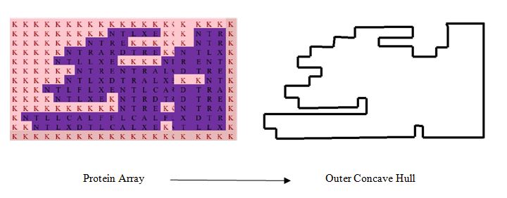
Figure 3. The concept of outer concave hull from the view point of protein array.
This section describes the proposed concave hull generation procedure. The procedure underlies four steps, as follows:
Step 1−creating an IFS fractal
To create an IFS fractal in the form of a point-cloud consisting of N + 1 points, {(x0,y0), (xi,yi) | i = 1,…,N}, an algorithm called IFS Algorithm can be used [12,13,17,18, 22], as follows.
IFS Algorithm:
|
|
|
Seed
|
(x0, y0)
|
|
|
Input
|
Number of Iterations
|
N
|
|
|
Mapping Parameters
|
(aj,bj,cj,dj,ej,fj), j = 1,...,n
|
|
|
|
|
|
|
|
Probabilities
|
(pj | j = 1,...,n)
|
|
|
|
|
|
|
|
Calculation
|
cpj =p1+...+pj, j = 1,...,n
|
|
|
|
w1
|
= [0,p1],...,wj = [cpj−1,cpj],...,wn = [cpn−1, cpn]
|
|
|
|
|
|
|
For i = 1,...,N
|
|
|
|
|
|
Generate a Random Number: ri ← [0,1]
|
|
|
|
|
If ri = w1 Then xi = a1xi−1 + b1yi−1 + e1, yi = c1xi−1 + d1yi−1 + f1
|
|
|
Iteration
|
|
…
|
|
|
|
|
|
|
|
|
|
|
If ri = wj Then xi = ajxi−1 + bjyi−1 + ej, yi = cjxi−1 + djyi−1 + fj
|
|
|
|
|
…
|
|
|
|
|
|
If ri = wn Then xi = anxi−1 + bnyi−1 + en, yi = cnxi−1 + dnyi−1 + fn
|
|
|
|
|
|
|
|
An IFS Algorithm has three segments, namely, Input, Calculation, and Iteration. In the Input segment four inputs items are set by the user, namely, Seed (x0, y0), Number of Iterations (N), Mapping Parameters ((aj,bj,cj,dj,ej,fj), j = 1,...,n), and Probabilities ((pj | j= 1,...,n)). The Calculation segment calculates the relative weights w1 = [0,p1],...,wj = [cpj−1,cpj],...,wn = [cpn−1, cpn] where cpj =p1+...+pj, j = 1,...,n, of the affine mappings needed to create points, {(xi,yi) | i = 1,…,N}. The Iteration segment creates the points {(xi,yi) | i = 1,…,N} in a recursive manner xi = ajxi−1 + bjyi−1 + ej, yi = cjxi−1 + djyi−1 + fj, j = 1,…,n, i = 1,…,N, preserving, at the same time, the relative weights of the affine mappings. It is worth mentioning that p1+...+pn = 1 and all affine mappings are contracting mappings. See [17,18] for the conditions needed for an affine mapping to be included in an IFS. In addition, in most cases, Seed (x0, y0) is equal to (0,0).
Step 2−Creating a binary array
In this step, a binary array BA = (…,bkl,…), ∀bkl ∈{0, 1}, is created from (xi,yi), i =0,…,N, i.e., from the point-cloud that models a fractal. To do this, a 2-dimentional grid is considered. To define the grid, the intervals xmin,…,xk,…,xmax and ymin,…,yl,…,ymax are needed where xmin ≤ min({xi | i = 0,…,N}), xmax ≥ max({xi | i = 0,…,N}), ymin ≤ min({yi | i = 0,…,N}), ymax ≥ max({yi | i = 0,…,N}), xk+1 = xk + x, k = 1,2,…,Nk, xk=0 = xmin, xk=Nk = xmax, yl+1 = yl + y, yl=0 = ymin, and yl=Nl = ymax.
It is worth mentioning that xmin, xmax, ymin, and ymax are user-defined values in accordance with the above conditions.
Step 3−Creating a protein array
In this step, the binary BA = (…,bkl,…) is transformed into a protein array using the DBC described in Section 2. The protein array is denoted as Protein = (…,Proteinij,…).
Needless to say, ∀Proteinij ∈ {A, C, D, E, F, G, H, I, K, L, M, N, P, Q, R, S, T, V, W, X, Y}.
Step 4−Recreating binary array
In this step, the protein array Protein is transformed into another binary array PB = (…,PBij,…) using a user-defined rule. The goal is to preserve the information of outer and inner segments of the fractal shape for generating the outer concave hull. For example, consider the arbitrary case shown in Figure 4. In this case, one can set a rule as follows: If Proteinij = K and Proteinij+1 = K, then PBij = 1; Otherwise PBij = 0. If this rule is applied to the protein array shown in Figure 4 (left-hand-side), then a binary array PB = (…,PBij,…) also shown in Figure 4 (right-hand-side) is produced. As observed from Figure 4, this binary array clearly distinguishes the outer boundary (given by the digit 1) from the inner boundary (given by the digit 0).
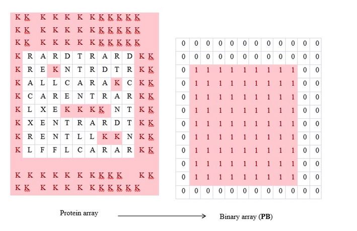
Figure 4. Significance of PB.
Step 5−Determination of Boundary Fence
This is the last step where the boundary fence array BF = (...,BFij,...) is determined by transforming the PB = (…,PBij,…). The goal is to find out the coordinates of the outer boundary fence. The procedure of getting PB = (…,PBij,…) is described as follows.
Let CM = {-1,0,1}×{-1,0,1}−{(0,0)} be a set and (p,q) be a member of it, i.e., (p,q) ∈ CM. Let BFij(p,q) be a binary digit, i.e, BFij(p,q) ∈ {0,1}, as defined by the equation (2).
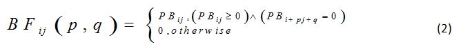
All possible values of BFij(p,q) can be added to determine the elements of PB. This yields equation (3), as follows
The coordinates of the elements corresponding to BFij > 0 represent the outer boundary fence or the outer concave hull. Figure 5 shows the BF = (...,BFij,...) that has been determined from the PB = (…,PBij,…) shown in Figure 4 using the procedure described above. One can observe from figure 5 that BFij > 0 clearly defines the required concave hull.
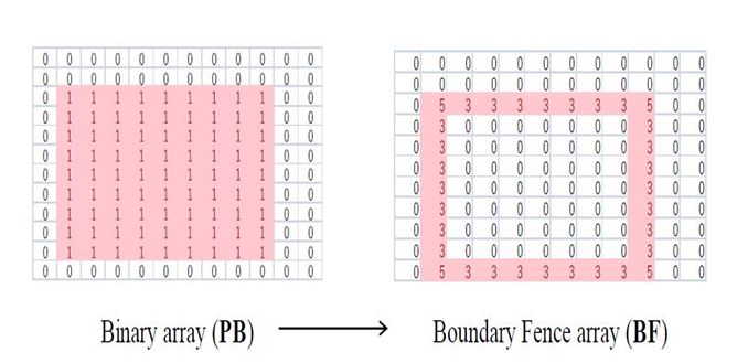
Figure 5. Significance of boundary fence array.
2021 Copyright OAT. All rights reserv
This section describes a case study where an IFS fractal modeling a snow crystal. The mapping parameters and the probabilities are shown in Table 2. As listed in Table 2, seven affine mappings are used to create the model of the snow crystal in terms of a point-cloud. The results obtained applying the Steps 1-5, as described in Section 3, are shown in Figure 6.
Table 2. Settings of IFS
Mapping |
|
|
|
Mapping Sets (i) |
|
|
Parameters |
1 |
2 |
3 |
4 |
5 |
6 |
7 |
|
|
|
|
|
|
|
|
ai |
0.5 |
0.33333 |
0.33333 |
0.33333 |
0.33333 |
0.33333 |
0.33333 |
bi |
-0.2887 |
0 |
0 |
0 |
0 |
0 |
0 |
|
|
|
|
|
|
|
|
ci |
0.28868 |
0 |
0 |
0 |
0 |
0 |
0 |
di |
0.5 |
0.33333 |
0.33333 |
0.33333 |
0.33333 |
0.33333 |
0.33333 |
ei |
0 |
0.57735 |
0 |
-0.5774 |
-0.5774 |
0 |
0.57735 |
fi |
0 |
0.33333 |
0.66667 |
0.33333 |
-0.3333 |
-0.6667 |
-0.3333 |
pi |
0.25 |
0.125 |
0.125 |
0.125 |
0.125 |
0.125 |
0.125 |
In particular, Figure 6a shows the point-cloud (the result of Step 1), Figure 6b shows the binary array (the result of Step 2), Figure 6c shows the protein array (the result of Step 3), Figure 6d shows the binary array called PB (the result of Step 4), Figure 6e shows the boundary fence array (the result of Step 5). As observed in Figures 6a-e, the outer and inner segments become distinguishable due to the application of the Steps 1-5 in a successive manner. A physical model has also been manufactured by an additive manufacturing equipment (a 3D printer), as shown in Figure 6f. In doing so, the outer concave hull shown in Figure 6e has been used to generate the STL data. The STL data generating process can be found in [16].
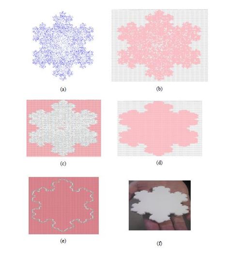
Figure 6. A case study of concave hull generation and physical model building.
This case study clearly demonstrates that the presented concave hull generation procedure is useful means to handle complex shapes for the sake of manufacturing their physical models.
Fractal geometry has extensively been used to quantify the complexity and normality/abnormality of the shapes observed in the living organisms (e.g., cell, tissue, lung, blood vassals, brain structures). These shapes are primarily represented by point-clouds having internal and external boundary fences (concave hulls). The extraction of these boundary fences is not an easy task. This study sheds some lights on this issue by proposing a simple but effective concave hull generating procedure where an in silico DNA-Based Computing plays an important role. It is demonstrated that the proposed concave hull generating procedure is able to create the outer boundary fence of a fractal (i.e., point-cloud created by an IFS) in a lucid manner. Further study can be carried out to generate the inner concave hulls of IFS fractals. Nevertheless, to get benefited from the capability of additive manufacturing in producing complex shapes having biomedical significance, the studies similar to this one must be continue in the years to come.
- Mandelbrot BB (1977) Fractals: form, chance, and dimension, W.H. Freeman and Co., San Francisco, CA.
- Mandelbrot BB (1982) The Fractal Geometry of Nature, W. H. Freeman: San Francisco.
- Barnsley MF (2012) Fractals Everywhere (New Edition), Dover Publications, Mineola, New York.
- Adamatzky A (2015) Slime mould processors, logic gates and sensors. Philos Trans A Math Phys Eng Sci 373. [Crossref]
- Park JS, Oha SJ (2012,2013) New Concave Hull Algorithm and Concaveness Measure for n-dimensional Datasets. Journal of Information Science and Engineering 28: 587-600, 29: 379-392.
- Asaeedi S, Didehvar F and Mohades A (2014) Alpha-Concave Hull, a Generalization of Convex Hull.
- Moreira AJC, Santos MY (2007) Concave hull: A k-nearest neighbours approach for the computation of the region occupied. In: Braz J, Vázquez PP, Pereira JM (Eds.), GRAPP 2007 - Proceedings of the Second International Conference on Computer Graphics Theory and Applications Volume GM-R March 8-11, 2007, Barcelona, Spain, 61-68, 2007.
- Xu, J, Feng Y, Zheng Z, Qing XA (2010) Concave Hull algorithm for scattered data and its applications, in Image and Signal Processing (CISP), 2010 3rd International Congress on, 5: 2430-2433.
- Chau AL, Li X and Yu W (2013) Convex and concave hulls for classification with support vector machine. Neurocomputing 122: 198-209.
- Vishwanath AV, Srivatsan RA, Ramanathan M (2013) Minimum area enclosure and alpha hull of a set of freeform planar closed curves. Computer-Aided Design 45: 751-763, 2013
- Vishwanath AV, Ramanathan M (2012) Concave Hull of a Set of Freeform Closed Surfaces in R3. Computer-Aided Design and Applications 9: 857-868.
- Ullah AMMS, Omori R, Nagara Y, Kubo A, Tamaki J (2013) Toward Error-Free Manufacturing of Fractals. Procedia CIRP 12: 43-48.
- Ullah AMMS, Sato Y, Kubo A, Tamaki J (2015) Design for Manufacturing of IFS Fractals from the Perspective of Barnsley's Fern-leaf. Computer-Aided Design & Applications 12: 241–255.
- Martyn T (2009) The attractor-wrapping approach to approximating convex hulls of 2D affine IFS attractors. Computers & Graphics 33: 104-112.
- Mishkinis A, Gentil C, Lanquetin S, Sokolov D (2012) Approximate convex hull of affine iterated function system attractors. Chaos, Solitons & Fractals 45: 1444-1451.
- Ullah AMMS, DʼAddona DM, Harib KH, Lin T (2016) Fractals and Additive Manufacturing. International Journal of Automation Technology 10.
- Barnsley MF, Demko S (1985) Iterated Function Systems and the Global Construction of Fractals. Proceedings of the Royal Society of London Series A: Mathematical and Physical Sciences 399: 243-275.
- Demko S, Hodges L, Naylor B (1985) Construction of fractal objects with iterated function systems. Computer Graphics 19: 271-278.
- ISO Standard (2013) Standard specification for additive manufacturing file format (AMF) Version 1.1, ISO/ASTM 52915:2013.
- Ullah AMMS (2015) Remodeling Fractals. Fractal Geometry and Nonlinear Analysis in Medicine and Biology 1.
- Ullah AMMS (2010) A DNA-Based Computing Method for Solving Control Chart Pattern Recognition Problems. CIRP Journal of Manufacturing Science and Technology 3: 293-303.
- Ullah AMMS, D'Addona D, Arai N (2014) DNA based computing for understanding complex shapes. Biosystems 117: 40-53.
- D'Addona DM, Ullah AMMS, Matarazzo D (2015) Tool-wear prediction and pattern-recognition using artificial neural network and DNA-based computing. Journal of Intelligent Manufacturing.
- Ullah AMMS (2015) In Silico DNA computing. International Journal of Swarm Intelligence and Evolutionary Computing 4: e111.
- Crick F (1970) Central Dogma of Molecular Biology. Nature 227: 561-563.