Take a look at the Recent articles

Abstract

In this paper, CS based medical images compression framework has been presented. The discrete cosine transform (DCT) as well as discrete wavelet transform (DWT) have been used for finding the sparsity in the medical images. The comparison of the results obtained by combining DCT and DWT with CS for medical images- CT and MRI- has been presented. The CS & DWT compression scheme achieved a maximum compression ratio (CR) of 3.01 with PSNR of 31.6732 dB and average CoC value of 0.9983 for an MRI image, whereas for CT image these values are 2.89, 31.7935 dB and 0.9987, respectively. The CS and DCT based algorithm could obtain a maximum CR value of 1.5789 with average values (for both types of images) of PSNR, RMSE and CoC of 13.1774 dB, 56.0007 and 0.8384, respectively.

Key words

Compressive sensing; discrete wavelet transform (DWT); discrete cosine transform (DCT); PSNR; RMS; CoC

Introduction

Nowadays, compression is a necessary step of images storage and transmission and Medical images contain huge and vital information. It is necessary to compress medical images without losing the vital data. So, for that we are using discrete cosine transform, discrete wavelet transform. Normally the Shannon/ Nyquist sampling theorem states that when capturing the signal one must sample at least two times faster than signal bandwidth to avoid losing information. In fact, this principle underlies nearly all signal acquisition protocol used in consumer audio, visual electronics, medical imaging devices, and radio receivers and so on. However, it is common in such systems to use an anti-aliasing low-pass filter to band limit the signal before sampling. Compressive Sensing is a new method to capture and represent the compressible signal at the rate significantly below the Nyquist rate. Compressive sensing theory asserts that one can recover certain signals or images from far fewer samples or measurements than traditionally required [1].

The concept of compressed sensing was originally presented by David Donoho in 2006 [2] which states that in a digital signal or image, if x is an unknown vector and we need to measure n linear functions of x and reconstruct the same. If x has “sparse” representation, which could be decided by some orthonormal basis like wavelet, Fourier or DCT, then x can be reconstructed by n samples (for a signal) or pixels (for an image) as opposed to a routine m samples/ pixel, where (n<<m). The concept was further elaborated and appled by Candes and Wakin in 2008 by representing the compressed sensing as compressive sampling, acquiring the signal/ image with sampling rate which is below Nyquist rate.

In [3-10] authors have used the above mentioned, concept of compressive sensing for compressing the medical images like CT, MRI etc. using various transforms. In this paper, we implemented the medical images-CT and MRI- compression using DCT, DWT and CS. The compression performance is evaluated using parameters like peak signal to noise ratio (PSNR), root mean square error (RMS) and correlation coefficient (CoC).

Compressive sensing

Using compressive sensing one can recover certain signals or images from far fewer samples than traditionally required [1]. Compressive sensing relies on two principles:

Sparsity- which pertains to the signals of interest, and Incoherence- which pertains to the sensing modality

Sparsity

A signal is called sparse if most of its components are zero. Sparsity expresses the idea that the “information rate” of a continuous time signal may be much smaller than suggested by its bandwidth, or that a discrete-time signal depends on a number of degrees of freedom which is comparably much smaller than its (finite) length [1].

As observed, many real-world signals are compressible in the sense that they are well approximated by sparse signal after an appropriate change of basis. However, a very good example of naturally sparse picture is the one of the sky during night, which has all pixels black except a few white dots (starts). Real world images are not usually sparse but can be translated into suitable domain to achieve sparsity. This explains why compression techniques such as JPEG, MPEG, or MP3 work so well in practice. For example, JPEG relies on the sparsity of images in the discrete cosine basis or wavelet basis and achieves compression by only storing the largest discrete cosine or wavelet coefficients.

For representing a signal in a sparse form, we would like to project it onto a convenient basis. The signal of interest x, having a sparse representation in some basis, Ψ = [.....] such that x =Ψs which can be mathematically expressed as

            (1)

Where “s” is the coefficient vector for “x” under the transformation basis Ψ.

Incoherence

This property demands that the measurement and sparsifying basis are incoherent i.e. the signal which has a sparse representation in a sparsifying basis must spread out in the measurement basis [1]. Within the Compressive sensing framework, low coherence between and translates to fewer samples required for reconstruction of signal. An example of low coherence measurement/representation basis pair is sinusoids and spikes that are incoherent in any dimension, and can be used for compressively sensing Signals having sparse representation in terms of sinusoids.

If our measurement matrix Ψ were a square matrix, then we may have employed an identity matrix for the sake of sampling the signals. Clearly, this is the case of our traditional uniform sampling. But there is no way to adjust an identity matrix for our measurement matrix since it is a short, fat matrix i.e. number of measurements M <<Signal length N.

Also, there must be least correlation between the elements of the sensing and the dictionary matrices as suggested by the incoherence property in section 2.3.2. The lesser the coherence between Ψ and Φ, fewer the number of measurements needed to recover the signal.

Mathematically, the coherence between the sensing basis Φ and the representation basis Ψ is given by [1]

            (2)

It follows from linear algebra that,

                         (3)

Here, µ indicates the correlation between the sensing matrix and the representation matrix. Lesser the value of coefficient of correlation, better the results in the sense that we need the acquisition of very lesser number of samples i.e. general linear measurements.

An example of low coherence measurement basis pair is sinusoids and spikes that are incoherent in any dimension, and can be used for compressively sensing Signals having sparse representation in terms of sinusoids [1]. Other common pairs are indicated in Table 1.

Table 1. Selection of Low coherence pairs

Φ	Ψ
Spike Basis	Fourier Basis
Spike Basis	Sinusoids
Noiselet	Wavelets
Gaussian or Binary _1	Any fixed

Recovery

Generally, L0, L1, L2 minimization methods are used for reconstruction. But if signal is sufficiently sparse then L1 minimization provides best solution [1].

We take l1-norm i.e. sum of absolute values of coefficients. We don’t pick a solution that is sparsest, or that has least energy. But we pick the one with smallest sum of magnitudes. Reason for doing this is that l1-norm is convex and hence, it becomes a linear programming problem and we get a lot of standard linear programming tools to solve it unlike l0-norm. Moreover, quite surprisingly, l1-norm gives almost the same result as the l0-norm [9].

Thus, the l1-norm essentially convexifies the l0-norm and is given as

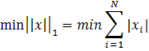            (4)

Wavelet transform

Previous we discuss that Medical images carry huge and vital information. It is necessary to compress the medical images without losing its vital-ness. Wavelet transform is preferable in the field of compression because of much more information of image can be retraced by it than any other transform [3]. There are many different types of wavelets have been used for compression and we have done quality analysis on reconstructed image.

Wavelet transform is a mathematical tool used to represent images in a domain in which it may be manipulated more effectively or in another word the main purpose of wavelet transform is to change the data from time-space domain to time-frequency domain which makes batter compression result.

The fundamental idea behind wavelets is to analyze the signal or image at different scales or resolutions, which is called multiresolution. Wavelets are a class of functions used to localize a given signal in both space and scaling domains. A family of wavelets can be constructed from a mother wavelet. Compared to Windowed Fourier analysis, a mother wavelet is stretched or compressed to change the size of the window. In this way, big wavelets give an approximate image of the signal, while smaller and smaller wavelets zoom in on details. Therefore, wavelets automatically adapt to both the high-frequency and the low-frequency components of a signal by different sizes of windows. Any small change in the wavelet representation produces a correspondingly small change in the original signal, which means local mistakes will not influence the entire transform.

Wavelet Transforms are based on small waves, called Wavelets, of varying frequency and limited duration. Wavelet analysis can be used to divide the information of an image into approximation and detail sub signals. The approximation sub signal shows the general trend of pixel values, and three detail sub signals show the vertical, horizontal and diagonal details or changes in the image. If these details are very small, then they can be set to zero without significantly changing the image [6].

As a result, there are 4 sub-band (A, H, V, D) images at each scale. The sub-band A is used for the next 2D DWT. The first, second and third level decomposition of image with the help of wavelet transform, here is showing first level of decomposition with four different frequency levels.

Now taken decomposition of A1 and achieved second level of decomposition and further got seven different frequency levels (Table 2).

Table 2. First level decomposition

A1	H1
V1	D1

And another time taken decomposition of A2 and achieved third level of decomposition and further got different frequency levels (Table 3).

Table 3. Second level decomposition

A2	H2	H1
V2	D2
V1		D1

Discrete cosine transform

A discrete cosine transform (DCT) expresses a finite sequence of data points in terms of a sum of cosine functions oscillating at different frequencies. The DCT is like the discrete Fourier transform: it transforms a signal or image from the spatial domain to the frequency domain.

DCT is a transform coding method comprising four steps. The source image is first partitioned into sub-blocks of size 8x8 pixels in dimension. Then each block is transformed from spatial domain to frequency domain using a 2-D DCT basis function. The resulting frequency coefficients are quantized and finally output to a lossless entropy coder. DCT is an efficient image compression method since it can decorrelate pixels in the image.

Here is the equation for 1- DCT

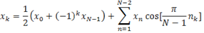            (5)

Where k = 0, 1 …..…N-1

Following is the equation for 2-DCT:

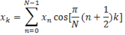                                     (6)

Here is the Figure 1 which gives the basic idea of DCT.

Figure 1. Discrete cosine transform

Table 4. Third level decomposition

A3	H3	H2	H1
V3	D3
V2		D2
V1			D1

Experimental results

In this section, the experimental (simulation) results for medical image compression using CS and DWT and CS and DCT has been presented. These algorithms are applied on a sample MRI (image 1) and CT (image 2) images, one each, and their performance is evaluated using PSNR, RMSE and CoC. All the simulations are performed using MATLAB software run on a core i7 CPU.

A.    CS and DWT based Results

(Figure 2, 3 and Table 5)

Figure 2. (a) Original image1 (b) CR=1.48 compressed image1 (c) CR=2.04 compressed image1 (d) CR=2.48 compressed image1 (e) CR=2.77 compressed image1 (f) CR=3.01 compressed image1

Figure 3. (a) Original image2 (b) CR=1.47 compressed image2 (c) CR=1.99 compressed image2 (d) CR=2.42 compressed image2 (e) CR=2.68 compressed image2 (f) CR=2.89 compressed image2

Table 5. Performance of CS and DWT based compression algorithm

	CR	PSNR, dB	RMS	CoC
Image 1	1.48	43.6326	1.6785	0.9998
	2.04	37.7404	3.3077	0.9992
	2.48	34.7934	4.6438	0.9984
	2.77	32.9042	5.7720	0.9975
	3.01	31.6732	6.6509	0.9966
Image2	1.47	44.0629	1.5973	0.9999
	1.99	38.2155	3.1316	0.9994
	2.42	35.1415	4.4613	0.9989
	2.68	33.2121	5.5711	0.9982
	2.89	31.7935	6.5594	0.9975

B.    CS and DCT based Results

Now the second method is use compressive sensing in discrete cosine transform. In this method, first we apply the discrete cosine transform and get the sparsity image then use this image in compressive sensing algorithm. In this algorithm first the set of sparse components are multiplied with the random Gaussian matrix. Here the size of Gaussian matrix is taken as M X N, where the M is taken as per the required percentage of measurement which is first generated randomly and finally converted to the orthogonal matrix. This matrix, multiplied with the sparse components, provides the set of compressed data of the image using compressed sensing. Now to reconstruct the set of data L1 minimization is used and reconstruct the image.

(Figures 4, 5 and Table 6)

Figure 4. (a) Original image1 (b) CR= 1.5789 compressed image1

Figure 5. (a) Original image2 (b) CR= 1.5789 compressed image2

Table 6. Performance of CS and DWT based compression algorithm

2021 Copyright OAT. All rights reserv

	CR	PSNR, dB	RMS	CoC
Image 1	1.5789	13.6059	53.2407	0.8487
Image 2	1.5789	12.7490	58.7608	0.8280

Conclusion

In this paper, a medical image compression framework using compressive sensing, discrete wavelet transform and discrete cosine transform has been presented. A sample CT and MRI image has been compressed using the algorithms combining CS & DWT and CS & DCT. Their performance is evaluated using PSNR, RMS and CoC parameters. The CS and DWT based compression algorithm outperforms the CS and DCT based algorithm as it achieved the highest compression ratio of 3.01 yielding the PSNR and CoC values of 31.6732 and 0.9966, respectively for an MRI image. For a CT image, this algorithm achieved a maximum PSNR and CoC values of 31.7935 and 0.9975, respectively while compressing the image with CR = 2.89. 

References

1. Candes E, Wakin M (2008) An introduction to Compressive Sampling. IEEE Signal Processing magazine 25: 21-30.
2. Donoho D (2006) Compressed sensing. IEEE Transactions on Information theory 52: 1289-1306.
3. Sapkal AM, Bairag VK (2009) Selection of Wavelets for medical image, Int. Conf. on Advances in Computing, Control and Telecommunication Technologies (ACT ’09) Trivandrum India. 678-680.
4. http://www-inst.eecs.berkeley.edu/~ee225b / sp11/ lectures/ CSmeetsML-Lecture1/ codes/ l1magic/ l1magic.pdf
5. Huihui B, Anhong W, Mengmeng Z (2010) Compressive Sensing for DCT Image. Int. Conf. on Computational Aspects of Social Networks (CASoN). 378-381.
6. Mayur MS, Falgun NT, Rahul KK, Chintan KM (2010) CT image compression using compressive sensing and wavelet transform. Int. Conf. on Communication Systems and Network Technologies (CSNT) 138-142.
7. Rabiul SI, Huang X, Keng LO (2015) Image Compression Based on Compressive Sensing Using Wavelet Lifting Scheme. The International Journal of Multimedia & its Applications 7: 1-16.
8. Qureshi MA, Deriche M (2016) A new wavelet based efficient image compression algorithm using compressive sensing. Multimedia Tools and Applications 75: 6737-6754.
9. Deriche M, Qureshi MA, Azeddine B (2015) An image compression algorithm using reordered wavelet coefficients with compressive sensing. International Conference on Image Processing Theory, Tools and Applications (IPTA) 498-503.
10. Shuling L, Baojun Z, Linbo T, Meiping J (2015) Adaptive image compression system based on TMS320C6713. IET International Radar Conference 1-5.