Abstract
The yellow-spined bamboo locust Ceracris kiangsu Tsai is a famous migratory forestry pest endemic to China. However, few genetic studies have been focusing on bamboo locusts. Here, we used microsatellite markers and the sequences from the mitochondrial COI gene to investigate genetic differences among the C. kiangsu populations from sampling locations of the species’ range in Southern China. High levels of genetic variation were determined for both mtDNA and microsatellites. For mtDNA data, there was a statistical support for a historical population increase for most populations except Jiangxi and Anhui, where no significant signals of expansion were detected. No significant isolation-by-distance pattern was observed by microsatellites data. Analyses of molecular variance indicated a consistent high level of differentiation within populations for COI and microsatellites, with FST = 0.27611 and FST = 0.20010 respectively. Phylogeographic analyses indicated little geographic structure, even though microsatellite-based Bayesian clustering identified two genetic clusters, suggesting a historically wide gene flow among the populations. The high levels of gene flow are likely to reflect the spread of this locust population into the surrounding areas. The lack of population structure in this species is likely caused by recent range expansions or cycles of local extinctions followed by recolonization/expansions. For the effective population size (Ne) in this locust, whether we used software ONeSAMP or LDNe, the results showed that Taoyuan population had a low Ne value, whereas GN had a high value. In general, its Ne s are 211, at a moderate level, by means of a global evaluation in all populations.
Key words
Ceracris kiangsu, population structure, mitochondrial sequences, microsatellites, genetic variability
Introduction
The yellow-spined bamboo locust Ceracris kiangsu Tsai is a famous migratory forestry pest endemic to China. It mainly distributes in South China and is characterised by its behavior of feeding in large groups on the leaves of bamboo plants during all of its life stages [1-3]. Due to this feeding habit, their distribution range is more restricted than Locust migratoria [4] and Oxya hylaintricate [5]. However, the C. kiangsu population has dramatically increased recently in many regions in China. Populations of herbivorous insects often fluctuate in response to host plant quality and availability [6,7].
Species with high migratory ability are usually supposed to have minimal population substructure over their distributional ranges because strong gene flow can counteract the isolating effects of geographical distance and physical barriers [8,9]. The current distribution of genetic variation within a species is the result of its demographic history as well as the interaction between mutation, genetic drift and gene flow. It is hard to distinguish historical effects, like climate change or geological accident, from shorter-term consequences of dispersal patterns and limited population size, but the distinction is important [10]. It is the effect of historical changes on the distribution and abundance of organisms left in the current population structure that underpins phylogeography [11]. Often these spatial genetic patterns are placed on a much larger scale than the correlations generated by dispersal of individuals in stable populations. There was defectiveness in prediction of the spread of agricultural pests and inferences about selection for local adaptation. It may be due to the traditional assumption that the current population structure was in equilibrium between drift, mutation and dispersal [10]. In these cases, historical effects may be considered a complicated factor.
The sensitivity to demographic fluctuations of statistics summarizing genetic variation is dependent on dispersal characteristics, effective population sizes, strength of demographic fluctuations, and properties of the genetic markers [12-14]. Population genetic structure can provide information to help evaluate the extent of the same potential evolutionary process and genetic differences among different populations, such as genetic drift, population range expansion or fragmentation [15]. Here, genomic data can help to uncover the degree of differentiation and the influence of historical events like climatic shifts and ecological changes. Furthermore, they may reveal patterns of geographic variation within the gene pool of a species or a species complex. To date, there have been a number of worldwide molecular studies on population structure and gene flow in locusts. Chapuis et al. [16] scored 14 microsatellites in 25 L. migratoria populations; the result rejected the hypothesis that L. migratoria consists of two genetically distinct clusters adapted to non-outbreaking or cyclically outbreaking. Chapuis et al. [17] analysed genetic variation within and between 24 population non-outbreaking populations and outbreaking populations in Western Europe, Madagascar and Northern China based on 14 microsatellites. The result showed that the long-term effective population size is similar in outbreaking and non-outbreaking populations with a similar genetic diversity, and FST values indicated that gene flow is substantially larger among outbreaking populations than among non-outbreaking populations. Ibrahim et al. [18] carried out a genetic survey in solitarious desert locust populations based on a single nuclear DNA marker. The study revealed a considerable genetic diversity within a population and substantial genetic variations among populations, despite the homogenizing potential of outbreak events. Most studies in the past were focused on the biological characteristic, morphological classification, disaster forecast and pest control for C. kiangsu. The latest genetic research has reported that C. kiangsu is a monophyletic group with a high level of genetic diversity, a low genetic differentiation among populations under the 16S rRNA and amplified fragment length polymorphism (AFLP) markers. It was a landmark of C. kiangsu in genetic research [9]. For this species, however, there is still a lack of any hypothesis about population substructure, population migration or mechanism of population outbreaking.
In this study, we first combined microsatellite and mitochondrial COI data to evaluate: (1) what is the degree of genetic diversity and variation? (2) whether microsatellite markers provided a favorable evidence for population structure which is not revealed by mtDNA markers, (3) are genetic differences consistent with geographic distances? and (4) if this species experienced a genetic bottleneck and/or a population explosion, what factors should be liable for it?
Material and methods
Sampling and dna extraction
Samples of C. kiangsu were collected in south and south-west of China. All samples were gathered in a period of five years. These sampling locations include Anhui, Fujian, Guangxi, Guangdong, Hunan, Jiangxi, Jiangsu, Sichuan, Sichuan, Yunnan and Zhejiang provinces. All specimens were preserved in 100% ethanol and stored at -20°C. Total DNA was extracted from individual hind legs, using the Genomic DNA Purification Kit (Promega, USA) following the user manual.
Mitochondrial DNA sequencing
We amplified the COI gene using primers described by Simon et al. [19] for 231 individuals from 12 geographical populations (Table 1). The reaction mixture (25 μL) contained 50 ng of DNA template, 2.5 μL of 10x buffer, 2 μL dNTP (2.0 mM), 2.5 μL MgCl2 (2.0 mM), 1. 5μL primers (10 μM) and 0.2μL rTaq DNA polymerase (5U/μL) (TaKaRa Biotechnology, Dalian, Liaoning, China). The thermal cycle profile was as the following: an initial denaturation of 2 min at 94°C; 35 amplification cycles of denaturation for 30 s at 94°C, annealing for 30 s at Tm and extension for 50 s at 72°C; and a final extension for 10 min at 72°C. PCR products were separated by 1% agarose gel, and PCR amplification products were performed by using ABI 373A automatic DNA sequencing (Applied Biosystems). Each fragment was sequenced in both directions, using the above primers and then aligned in the software MEGA 6 [20].
Microsatellites
Ten microsatellites, WJ621, WJ622, WJ623, WJ624, WJ625, WJ626, WJ627, WJ630, WJ631 and WJ632 [3] were examined in this study. Samples in this part were different from the samples for COI gene. Here we used 433 individuals for genotyping in 18 sampling sites (Table 1). PCR amplifications were performed in a total volume of 15 μL containing 20 ng of template genomic DNA, 0.1 μmol/L of each primer (forward and reverse), 1 × PCR buffer, 0.2 mmol/L dNTPs, and 0.5 units of TaKaRa Taq (Takara Bio, Shiga, Japan) with the following cycling profile: 15 min at 94°C; 35 cycles of 30 s at 94°C, annealing for 30 s (Annealing temperature see Table 2), and extension at 72°C for 30 s, and an 10 min final extension step. ABI 3500XL Genetic Analyzer (Applied Biosystems, Foster City, CA) was used to analyse the amplified PCR products, and GeneMapper version 3.5 software (Applied Biosystems, Foster City, Calif) was used to obtain allele designations.
Table 1. All samples used in microsatellite and mtDNA analysis. N is the total number of individual used in this study, NSSR is the number of individual used for microsatellite genotyping, NmtDNA is the numer of individual used for COI sequencing
Code |
County, Province |
N |
NSSR |
NmtDNA |
Coordinates |
SC |
Changing, Sichuan |
20 |
20 |
20 |
28°34′56″N/104°55′16″E |
HC |
Jinyun, Chongqing |
20 |
20 |
20 |
29°52′04″N/106°21′06″E |
RA |
Rongan, Guangxi |
20 |
20 |
20 |
25°17′32″N/109°32′21″E |
BG |
Quanzhou, Guangxi |
20 |
20 |
19 |
25°55′43″N/111°04′22″E |
SP |
Shuangpai, Hunan |
20 |
20 |
- |
25°57′42″N/111°39′35″E |
GN |
Guangning, Guangdong |
35 |
35 |
27 |
23°38′04″N/112°26′26″E |
JX |
Shicheng, Jiangxi |
20 |
20 |
15 |
26°19′35″N/116°20′36″E |
FJ |
Jianou, Fujian |
15 |
15 |
12 |
27°01′21″N/118°18′17″E |
QZ |
Quzhou, Zhejiang |
15 |
15 |
14 |
28°58′06″N/118°52′16″E |
GD |
Guangde, Anhui |
15 |
15 |
- |
30°54′17″N/119°33′51″E |
ZJ |
Nanjing, Jiangsu |
33 |
33 |
20 |
32°04′14″N/118°50′57″E |
AH |
Shucheng, Anhui |
20 |
20 |
16 |
31°20′08″N/116°37′55″E |
WH |
Wuhan, Hubei |
35 |
35 |
|
30°37′41″N/114°18′11″E |
HR |
Huarong, Hunan |
20 |
20 |
18 |
29°31′51″N/112°32′25″E |
TY |
Taoyuan, Hunan |
35 |
35 |
30 |
28°54′09″N/111°29′20″E |
AA |
Anhua, Hunan |
35 |
35 |
- |
28°13′48″N/111°07′12E |
TJ |
Taojiang, Hunan |
20 |
20 |
- |
28°34′5″N/112°09′43″E |
CS |
Changsha, Hunan |
35 |
35 |
- |
28°15′0″N/112°55′55″E |
Total |
- |
433 |
433 |
231 |
- |
Table 2. Samples sites, number of samples(N), number of haplotypes (h), haplotype diversity (Hd), nucleotide diversity (π), Fu’s Fs and Tajima's D, SSD (Sum of Squared deviation), HRI (Harpending’s Raggedness index), tau (τ) and theta at time 0 and 1 (θ0 and θ1) of COI for Ceracris kiangsu.
Code |
N |
h |
Hd |
π |
Fu’s Fs |
Tajima's D |
SSD |
HRI |
τ-values |
θ0 |
θ1 |
AH |
16 |
16 |
1.000 |
0.0419 |
-3.622 |
-0.6573 |
0.0112 |
0.0122 |
3.180 |
6.479 |
99999.000 |
HC |
20 |
6 |
0.516 |
0.001 |
-2.743** |
-1.5703* |
0.0112 |
0.1047 |
1.865 |
0.000 |
1.227 |
FJ |
12 |
7 |
0.773 |
0.002 |
-3.413** |
-1.3042 |
0.0148 |
0.0888 |
0.742 |
0.980 |
99999.000 |
GN |
27 |
25 |
0.991 |
0.027 |
-8.367** |
-0.9176 |
0.0064 |
0.0105 |
10.133 |
5.214 |
29.617 |
GX |
19 |
19 |
1.000 |
0.016 |
-10.613** |
-0.0677 |
0.0031 |
0.0053 |
5.500 |
7.555 |
233.438 |
HR |
18 |
10 |
0.863 |
0.006 |
-1.923 |
-2.2334** |
0.0099 |
0.0640 |
1.690 |
0.000 |
99999.000 |
JX |
15 |
10 |
0.895 |
0.011 |
-0.802 |
1.2130 |
0.0340 |
0.1079 |
5.479 |
3.777 |
27.173 |
QZ |
14 |
12 |
0.967 |
0.007 |
-6.047** |
-0.6144 |
0.0093 |
0.0366 |
2.660 |
2.288 |
505.625 |
RA |
20 |
12 |
0.889 |
0.006 |
-3.892* |
-1.4575 |
0.0125 |
0.0383 |
0.570 |
2.816 |
99999.000 |
SC |
20 |
7 |
0.584 |
0.001 |
-4.000** |
-2.0409** |
0.0004 |
0.0450 |
0.975 |
0.077 |
4.270 |
TY |
30 |
8 |
0.715 |
0.002 |
-3.414* |
-0.7096 |
0.0047 |
0.0886 |
1.174 |
0.000 |
99999.000 |
ZJ |
20 |
8 |
0.805 |
0.002 |
-3.539** |
-1.2670 |
0.0049 |
0.0869 |
1.479 |
0.000 |
99999.000 |
Total |
231 |
113 |
0.9322 |
0.014 |
-34.373 |
-2.3016** |
0.0102 |
0.0578 |
2.954 |
2.4321 |
50066.279 |
Mitochondrial data analysis
Sequence alignments of mtDNA data were performed using MEGA 6 [20]. Haplotype and nucleotide diversities were calculated with DNASP 5 [21]. We constructed median joining haplotype network with Network 4.611 [22] and used the MEGA6 under kimura 2-parameter model to generate a bootstrap tree.
Genetic differentiations within and among populations were measured by analysis of molecular variance (AMOVA) based on traditional F-statistics with 10,000 permutations in Arlequin V3.5 [23]. The demographic histories were examined with Tajima’s D and Fu’s F neutrality tests [24,25] using 1,000 simulation steps as implemented in Arlequin V3.5. In these tests, negative significant deviations from neutrality might indicate either balancing selection or population expansion.
Microsatellites data analysis
Allele frequency, number of alleles, observed and expected heterozygosities, FST [26] and Nei’s [27] unbiased genetic distances were calculated, using Genetix 4.02 software [28] and POPGENE version 1.3.1 [29]. We did tests for deviation from Hardy–Weinberg equilibrium (HWE) at each locus for each population and genotypic linkage disequilibrium among loci, using a Markov Chain Monte Carlo method performed in Genepop version 3.4 [30], and then used sequential Bonferroni correction to correct P values [31]. An overall inbreeding coefficient (FIS) [26] was also of the view to measure the HWE departures by evaluating the probabilities through random permutation procedures (minimum 10,000 permutations). Significant value associated with the HWE analysis was adjusted following sequential Bonferroni procedures [31].
We applied a Bayesian analysis implemented in the program in the STRUCTURE program [32,33] for estimating hidden substructure across the studied species’ range of C. kiangsu. This program generated clusters of individuals based on their multilocus genotypes. An admixture ancestry model and the correlated allele frequency model were used to calculate the probable number of genetic clusters (K) with a burn-in period of 100 000 iterations and 1 000 000 Markov chain Monte Carlo (MCMC) repetitions. We performed 10 independent runs for each K to confirm consistency across runs, tested K from 1 to 10 and used ΔK method of Evanno et al. [34] to choose the most likely value of K.
We used the ARLEQUIN version 3.0 [35] to conduct the analysis of molecular variance (AMOVA). We defined the population structure on the basis of phylogenetic clusters which we obtained from the STRUCTURE program. We carried out a hierarchical analysis of variance to partition total variance into variance components attributable to interindividual and/or interpopulation differences. Pairwise estimates of FST were transformed into pairwise estimates of gene flow Nm among populations, again using ARLEQUIN. We also used the Mantel test to evaluate the correlation between FST and geographical distance at Isolation By Distance Web Service Version 3.23 [36]. Next, we also used the program ONeSAMP with approximate Bayesian computation method to estimate Ne, the effective population number [37]. We set the prior (lower and upper bounds) on Ne at 10 and 10000 (In order to obtain accurate results, we used populations which individual number ≥30). As a comparison, we also applied the program LDNe to estimate Ne based on linkage disequilibrium [38].
Results
Mitochondrial DNA data
Overall, 231 COI fragment sequences covered 671 base pairs (bp) (GenBank Accession no: KJ667224 - KJ667509). The average nucleotide frequencies of adenine (A), thymine (T), guanine (G) and cytosine (C) were 32.0%, 33.2%, 16.7%, and 18.1%, respectively. Of the 231 COI fragments sequences, 178 polymorphic sites were observed, and 113 haplotypes were defined. Of the 178 sites, 43 were single variable sites, 135 were parsimony-information sites, and insertions or deletions were not observed in the examined sequences. The number of haplotypes, the values of haplotype diversity and nucleotide diversity within each and the total population were presented in Table 2.
The test of neutrality based on 1000 simulating samplings was negative in all populations, and in HR and SC significantly negative. The populations of all sample sites were also significantly negative, with Tajima's D value of -2.30157, P < 0.01 and Fu’s Fs value of -34.373, P<0.1. Harpending’s Raggedness index (HRI) = 0.05799, P>0.1. The negative value of Fu’s Fs and Tajima's D commonly indicate that the populations have been through a population expansion. Large differences between θ0 and θ1 within all collections indicate a rapid population expansion. The τ-values varied among all populations, indicating that the population expansions date back to very wordy time period. The τ-value for the pooled sequences was calculated to be 2.954. We used the τ=2ut (t is population expansion time, u is nucleotide mutation rate per sequence per generation), u=2μk (μ is mutation rate of each nucleotide). Here, we used μ=2.30% per million years of Melanoplus [39] to calculate the population expansion time for C. kiangsu and got a t value of 0.0478.
The NJ tree of COI haplotypes observed in this study was shown in Figure 1. All haplotypes in the figure were split into three clades. However, haplotypes in 12 populations were disordered. Such as, the Anhui population consist of 16 individuals, which belongs to 16 haplotypes; In the Figure 1, Clade 1 included two haplotypes, Hap2 (AH11) and Hap5 (AH15); Clade 2 included two haplotypes, Hap50 (GN38) and Hap51 (GN40); the rest of others fall into Clade 3. The COI haplotype network did not show a clear genetic division. Close genetic relationship occurred throughout all populations with highly shared haplotypes among all populations (Figure 2). 113 haplotypes contacted with each other through mutations and formed a complex network.
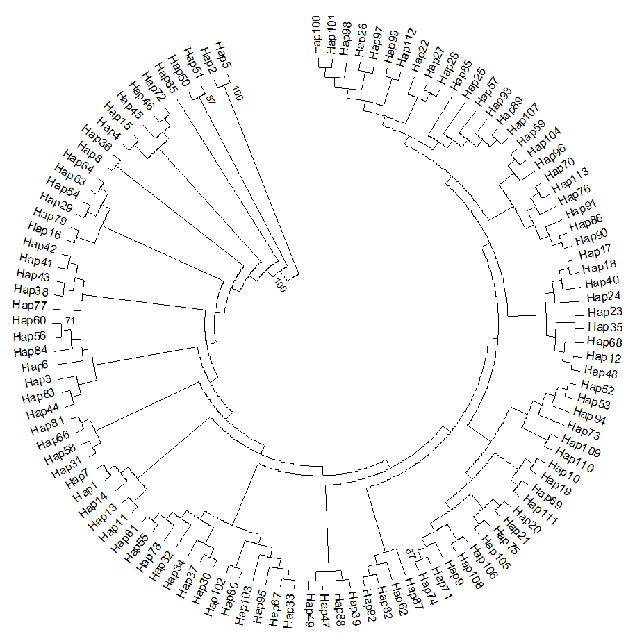
Figure 1. Neighbour-joining phylogenetic tree of mtDNA COI haplotypes in C. kiangsu population. The tree was rooted using midpoint rooting.

Figure 2. Median-joining networks showed genetic relationship among haplotypes of mtDNA COI gene for12 C. kiangsu populations
Most pair-wise FST values between populations were quite high and significant for the COI locus, with the exception of the AH/GN, AH/JX, HR/CH, SC/CH, JX/GN, JX/GX, SC/HR, ZJ/HR comparisons (FST<0.1) (Table 3). Population specific FST ranged from 0.16161 to 0.30923. Given that all groups have a common ancestral population, these population specific coefficients FST would represent the degree of evolution of particular populations from a common ancestral population. The pair-wise population FST ranged from -0.01107 to 0.49338, indicating a difference fromdifferentiations.
Statistical significance: *, P < 0.05, **, P < 0.01
Table 3. Pair-wise difference (FST) of 12 populations of C. kiangsu (below the diagonal) and population specific FST
pop |
Specific FST |
AH |
CH |
FJ |
GN |
GX |
HR |
JX |
QZ |
RA |
SC |
ZJ |
AH |
0.16161 |
|
|
|
|
|
|
|
|
|
|
|
CH |
0.30923 |
0.39522 |
|
|
|
|
|
|
|
|
|
|
FJ |
0.30575 |
0.29603 |
0.49338 |
|
|
|
|
|
|
|
|
|
GN |
0.21250 |
0.03816 |
0.33849 |
0.24202 |
|
|
|
|
|
|
|
|
GX |
0.25386 |
0.06300 |
0.41706 |
0.33724 |
0.11650 |
|
|
|
|
|
|
|
HR |
0.29128 |
0.31800 |
0.04182 |
0.22292 |
0.26364 |
0.29001 |
|
|
|
|
|
|
JX |
0.27304 |
0.08766 |
0.44502 |
0.32260 |
0.02287 |
-0.01107 |
0.28804 |
|
|
|
|
|
QZ |
0.28952 |
0.23810 |
0.41917 |
0.13178 |
0.15893 |
0.21392 |
0.23391 |
0.14881 |
|
|
|
|
RA |
0.29284 |
0.27749 |
0.44114 |
0.22830 |
0.21464 |
0.27962 |
0.27615 |
0.25424 |
0.21206 |
|
|
|
SC |
0.30905 |
0.39497 |
-0.01591 |
0.48018 |
0.33759 |
0.41420 |
0.02907 |
0.44192 |
0.40763 |
0.43672 |
|
|
TY |
0.30758 |
0.45437 |
0.17401 |
0.43662 |
0.37922 |
0.45476 |
0.02144 |
0.48636 |
0.42447 |
0.44206 |
0.16192 |
|
ZJ |
0.30622 |
0.37602 |
0.19173 |
0.14333 |
0.30890 |
0.39233 |
0.07847 |
0.38905 |
0.24525 |
0.30406 |
0.17751 |
0.16774 |
The AMOVA test of COI data disclosed that 27.61% occurred among populations within a group with a FST = 0.27611 (p = 0.000), and 72.39% of the genetic variations occurred within a population, showing a high level of variations within a population. According to the Neighbour-joining phylogenetic tree of COI haplotypes, we grouped all populations into three groups, i.e. group 1(GN), group 2(AH), and group 3 for the AMOVA test (Table 4). The results showed that a larger percent of variations within a population and the fixation indexes in each level were moderate.
Non-significant values are in bold; all other values are highly significant (P< 0.001).
Table 4. Hierarchical analysis of molecular variance (AMOVA) based on mtDNA
Classify |
Source of variation |
Sum of squares (d.f.) |
Percentage of variation |
Fixation index |
1 |
Among populations |
315.062 (11) |
27.61 |
FST = 0.276 (p<0.0001) |
|
Within populations |
755.804(219) |
72.39 |
|
|
Among groups |
169.212 (2) |
30.43 |
FSC=0.165 (P<0.0001) |
2 |
Among populations within groups |
145.849(9) |
11.49 |
FCT=0.304 (P<0.05) |
|
Within populations |
755.804(219) |
58.08 |
FST=0.419 (P<0.0001) |
Microsatellite data
Genotypes analysis of 433 individuals of C. kiangsu revealed a diverse degree of polymorphism across the 18 sampled locations. All loci showed significant deviation from HWE. There was no evidence of significant levels of linkage disequilibrium for multiple comparisons in the pooled data. The observed allele number per location ranged from 8.2 to 18.8. The number of effective alleles ranged from 4.9779 to 12.8480. All 10 microsatellite loci tested were polymorphic with PIC value ranged from 0.528 to 0.941. Mean HO and HE for each locus were 0.7100 and 0.9465, respectively. The average HO per sampling site ranged from 0.5600 to 0.8543 with the lowest value in the sample from GD (Anhui province) and the highest value in the sample from AA (Hunan province). The average HE per sampling site ranged from 0.7636 to 0.9143 ± 0.0312 with the lowest value in the sample from GD (Anhui province) and the highest value in the sample from TY (Hunan province). FIS (inbreeding coefficient) is the proportion of variance in the subpopulation contained in an individual. FIS value ranged from -0.01084 (AA) to 0.31436 (BG). High FIS indicated a high degree of inbreeding among individuals within populations (Table 5).
Table 5. Diversity indexes for 18 populations of C. kiangsu in 10 SSRs. Expected (HE) and observed (HO) heterozygosity are presented with standard errors. (NA: number of alleles, Ne: number of effective alleles, FIS: inbreeding coefficient)
location |
NA |
Ne |
HO (SD) |
HE (SD) |
FIS |
SC |
10.5000 |
6.7499 |
0.6950±0.1641 |
0.8205±0.0912 |
0.17790 |
HC |
11.2000 |
7.1369 |
0.6900±0.1883 |
0.8375±0.0616 |
0.20085 |
RA |
13.4000 |
9.3815 |
0.7100±0.1410 |
0.8729±0.0677 |
0.21123 |
BG |
11.6000 |
8.0679 |
0.6150±0.1811 |
0.8675±0.0423 |
0.31436 |
SP |
12.6000 |
7.7401 |
0.7000±0.1394 |
0.8443±0.0729 |
0.19565 |
GN |
18.3000 |
11.6944 |
0.7343±0.0842 |
0.9087±0.0255 |
0.20589 |
JX |
14.0000 |
9.1800 |
0.6700±0.1085 |
0.8759±0.0489 |
0.25913 |
FJ |
10.5000 |
7.3769 |
0.6333±0.1482 |
0.8480±0.0663 |
0.28514 |
QZ |
11.8000 |
7.8891 |
0.6667±0.2177 |
0.8404±0.0802 |
0.23954 |
GD |
8.2000 |
4.9779 |
0.5600±0.2089 |
0.7636±0.1033 |
0.29833 |
ZJ |
15.3000 |
9.6681 |
0.7455±0.1727 |
0.8898±0.0266 |
0.17713 |
AH |
12.0000 |
7.7887 |
0.7200±0.1274 |
0.8599±0.0442 |
0.18753 |
WH |
14.9000 |
8.4790 |
0.7229±0.0701 |
0.8549±0.0774 |
0.16857 |
HR |
14.5000 |
9.1811 |
0.7650±0.1415 |
0.8806±0.0391 |
0.15641 |
TY |
18.8000 |
12.8480 |
0.7600±0.1612 |
0.9143±0.0312 |
0.18283 |
AA |
12.1000 |
6.8011 |
0.8543±0.0966 |
0.8332±0.0604 |
-0.01084 |
TJ |
13.1000 |
8.8392 |
0.7150±0.0709 |
0.8778±0.0376 |
0.21006 |
CS |
15.4000 |
9.4921 |
0.6229±0.1269 |
0.8842±0.0416 |
0.30871 |
Nei's unbiased genetic distances and FST value for all the population pairs were estimated (Table 6). Genetic distance varied from 0.2880 between WH and CS to 2.4410 between TJ and SC. In brief, FST values ranged from 0.0177 (HR-RA) to 0.1561 (GD-SC). FST values for most breed combinations were greater than 0.01 indicated little and moderate differentiation between populations, suggesting a close genetic association among all populations. Gene flow among all populations is shown in Table 7. Nm value ranged from 1.41 (SC-GD) to 18.8 (RA-HR).
Table 6. FST value (below diagonal), Nei's (1978) unbiased genetic distance (above diagonal) of all population pairs
|
SC |
HC |
RA |
BG |
SP |
GN |
JX |
FJ |
QZ |
GD |
ZJ |
AH |
WH |
HR |
TY |
AA |
TJ |
CS |
SC |
|
0.5660 |
0.6939 |
0.9729 |
2.3542 |
1.1114 |
1.0566 |
1.0715 |
0.9370 |
1.7913 |
0.7133 |
0.6695 |
2.3172 |
0.5718 |
0.5735 |
2.0015 |
2.4410 |
1.6279 |
HC |
0.0646 |
|
0.6103 |
0.5172 |
2.0266 |
0.7995 |
0.7646 |
0.7483 |
0.9207 |
1.7637 |
0.6218 |
0.4896 |
2.0475 |
0.6518 |
0.5669 |
2.0038 |
1.8435 |
1.4004 |
RA |
0.0662 |
0.0547 |
|
0.5866 |
1.9180 |
0.5928 |
0.6784 |
0.6884 |
0.7247 |
1.7768 |
0.6689 |
0.3040 |
2.0322 |
0.2825 |
0.5020 |
1.9710 |
1.9179 |
1.6636 |
BG |
0.0847 |
0.0485 |
0.0443 |
|
1.6899 |
0.5843 |
0.3473 |
0.7285 |
0.8362 |
1.8435 |
0.6083 |
0.4038 |
2.0234 |
0.5813 |
0.6396 |
1.9338 |
1.5670 |
1.4221 |
SP |
0.1333 |
0.1203 |
0.1023 |
0.1001 |
|
1.0558 |
1.3446 |
2.0108 |
2.2755 |
0.7665 |
1.3095 |
1.7492 |
0.2182 |
1.6925 |
0.9362 |
0.4715 |
0.3053 |
0.3934 |
GN |
0.0807 |
0.0608 |
0.0384 |
0.0395 |
0.0693 |
|
0.6059 |
0.7144 |
0.9783 |
1.3161 |
0.5418 |
0.6715 |
0.8929 |
0.6803 |
0.4938 |
0.8955 |
0.8598 |
0.7187 |
JX |
0.0861 |
0.0642 |
0.0478 |
0.0252 |
0.0874 |
0.0382 |
|
0.9672 |
0.9926 |
1.7883 |
0.7305 |
0.4847 |
1.7530 |
0.5268 |
0.7521 |
1.5160 |
1.6396 |
1.4054 |
FJ |
0.0936 |
0.0683 |
0.0535 |
0.0575 |
0.1117 |
0.0493 |
0.0678 |
|
0.5614 |
1.7117 |
0.5920 |
0.7316 |
1.9950 |
0.5300 |
0.7205 |
1.5715 |
1.7891 |
1.3700 |
QZ |
0.0888 |
0.0815 |
0.0581 |
0.0664 |
0.1192 |
0.0641 |
0.0717 |
0.0500 |
|
1.7010 |
0.5626 |
0.7193 |
1.8962 |
0.6219 |
0.7045 |
1.4688 |
1.8491 |
1.5068 |
GD |
0.1561 |
0.1476 |
0.1323 |
0.1362 |
0.0956 |
0.1071 |
0.1313 |
0.1391 |
0.1421 |
|
1.6180 |
1.8153 |
0.7302 |
1.7176 |
1.1730 |
1.0646 |
0.9671 |
0.9823 |
ZJ |
0.0661 |
0.0546 |
0.0470 |
0.0449 |
0.0844 |
0.0347 |
0.0495 |
0.0462 |
0.0463 |
0.1233 |
|
0.5182 |
1.0710 |
0.4378 |
0.4306 |
0.9559 |
0.9841 |
0.8346 |
AH |
0.0677 |
0.0477 |
0.0231 |
0.0332 |
0.1047 |
0.0466 |
0.0382 |
0.0600 |
0.0615 |
0.1390 |
0.0410 |
|
1.8282 |
0.3325 |
0.3585 |
1.8527 |
1.9169 |
1.4238 |
WH |
0.1318 |
0.1201 |
0.1043 |
0.1065 |
0.0217 |
0.0638 |
0.0981 |
0.1113 |
0.1127 |
0.0922 |
0.0767 |
0.1064 |
|
1.9109 |
0.7286 |
0.3573 |
0.3354 |
0.2880 |
HR |
0.0554 |
0.0558 |
0.0177 |
0.0421 |
0.0945 |
0.0407 |
0.0362 |
0.0406 |
0.0494 |
0.1276 |
0.0304 |
0.0247 |
0.0990 |
|
0.5735 |
1.9009 |
1.7597 |
1.4374 |
TY |
0.0526 |
0.0466 |
0.0321 |
0.0413 |
0.0630 |
0.0266 |
0.0441 |
0.0483 |
0.0500 |
0.1002 |
0.0272 |
0.0260 |
0.0547 |
0.0340 |
|
0.6156 |
0.8891 |
0.6126 |
AA |
0.1372 |
0.1298 |
0.1139 |
0.1155 |
0.0545 |
0.0721 |
0.1026 |
0.1123 |
0.1121 |
0.1232 |
0.0801 |
0.1172 |
0.0437 |
0.1093 |
0.0560 |
|
0.5117 |
0.3451 |
TJ |
0.1185 |
0.1019 |
0.0870 |
0.0827 |
0.0257 |
0.0496 |
0.0807 |
0.0922 |
0.0967 |
0.0997 |
0.0604 |
0.0929 |
0.0304 |
0.0809 |
0.0491 |
0.0519 |
|
0.3190 |
CS |
0.1057 |
0.0925 |
0.0843 |
0.0809 |
0.0362 |
0.0457 |
0.0771 |
0.0838 |
0.0906 |
0.1007 |
0.0562 |
0.0840 |
0.0279 |
0.0761 |
0.0392 |
0.0385 |
0.0230 |
|
The STRUCTURE software, which analyzes genetic structure through a Bayesian approach, showed that the number of genetic groups (K value) best fitting our data was K = 2, with most individuals from the SC, TY, AH, RA, HR, ZJ, GN, JX, BG, HC, QZ and FJ populations included in Group I, while most individuals from CS, GD, SP, TJ, WH and AA populations included in the Group II. This indicated that populations of C. kiangsu consist of two genetically differentiated groups (Figure 3). It is to be noted that TY, ZJ, and GN populations consist of two groups, indicating a frequent gene exchange. Mantel tests revealed that there was not evident relationship between geographical and genetic distance (FST), R2= 0.0288, P = 0.1040 (Figure 4).
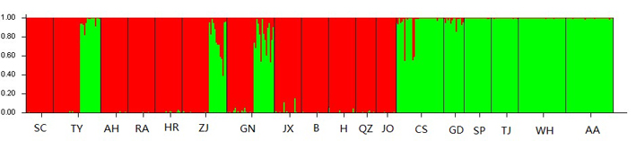
Figure 3. Two clades results from Bayesian cluster analyses of C. kiangsu. The number of optimal cluster (K) was two when calculated in STRUCTURE 2.1

Figure 4. The correlation analysis of genetic and geographic distance of C. kiangsu populations. Abscissa is the geographic distance, ordinate is the FST value
The results of AMOVA, based on the groups obtained from structure analysis, indicated that the greatest percentage of variation (97.72%) was contained within a population, 5.93% of the variance was among populations within a group, and 1.35% of the variance was among groups (Table 8). There was a significant genetic differentiation (FST = 0.20010, P < 0.01) within a population, based on FST estimates for hierarchical levels analyzed.
Table 7. Nm value between all populations of Ceracris kiangsu (above diagonal)
| |
SC |
HC |
RA |
BG |
SP |
GN |
JX |
FJ |
QZ |
GD |
ZJ |
AH |
WH |
HR |
TY |
AA |
TJ |
CS |
SC |
|
3.91 |
3.81 |
2.92 |
1.68 |
2.99 |
2.84 |
2.61 |
2.75 |
1.41 |
3.73 |
3.70 |
1.69 |
4.61 |
4.83 |
1.58 |
1.94 |
2.22 |
HC |
|
|
4.78 |
5.67 |
1.91 |
4.14 |
4.01 |
3.81 |
3.06 |
1.52 |
4.65 |
5.56 |
1.89 |
4.60 |
5.56 |
1.69 |
2.32 |
2.60 |
RA |
|
|
|
6.35 |
2.31 |
7.01 |
5.69 |
5.12 |
4.57 |
1.74 |
5.52 |
13.56 |
2.22 |
18.80 |
8.56 |
1.97 |
2.80 |
2.90 |
BG |
|
|
|
|
2.40 |
6.94 |
13.62 |
4.86 |
4.02 |
1.70 |
5.92 |
9.01 |
2.19 |
6.64 |
6.52 |
1.95 |
3.02 |
3.07 |
SP |
|
|
|
|
|
3.56 |
2.80 |
2.12 |
1.95 |
2.55 |
2.83 |
2.24 |
13.46 |
2.51 |
3.95 |
4.44 |
11.84 |
7.79 |
GN |
|
|
|
|
|
|
7.11 |
5.43 |
3.97 |
2.20 |
7.57 |
5.59 |
3.83 |
6.49 |
10.22 |
3.28 |
5.22 |
5.67 |
JX |
|
|
|
|
|
|
|
3.90 |
3.61 |
1.76 |
5.24 |
7.39 |
2.39 |
7.78 |
5.99 |
2.22 |
3.08 |
3.23 |
FJ |
|
|
|
|
|
|
|
|
5.79 |
1.67 |
5.81 |
4.42 |
2.09 |
6.98 |
5.51 |
2.01 |
2.67 |
2.99 |
QZ |
|
|
|
|
|
|
|
|
|
1.61 |
5.74 |
4.24 |
2.05 |
5.44 |
5.25 |
2.01 |
2.51 |
2.72 |
GD |
|
|
|
|
|
|
|
|
|
|
1.86 |
1.63 |
2.60 |
1.80 |
2.36 |
1.81 |
2.44 |
2.41 |
ZJ |
|
|
|
|
|
|
|
|
|
|
|
6.42 |
3.11 |
8.98 |
9.90 |
2.92 |
4.15 |
4.49 |
AH |
|
|
|
|
|
|
|
|
|
|
|
|
2.17 |
12.00 |
10.89 |
1.90 |
2.58 |
2.91 |
WH |
|
|
|
|
|
|
|
|
|
|
|
|
|
2.35 |
4.53 |
5.62 |
9.07 |
9.91 |
HR |
|
|
|
|
|
|
|
|
|
|
|
|
|
|
7.91 |
2.06 |
3.01 |
3.25 |
TY |
|
|
|
|
|
|
|
|
|
|
|
|
|
|
|
4.31 |
5.25 |
6.72 |
AA |
|
|
|
|
|
|
|
|
|
|
|
|
|
|
|
|
4.69 |
6.62 |
TJ |
|
|
|
|
|
|
|
|
|
|
|
|
|
|
|
|
|
13.85 |
CS |
|
|
|
|
|
|
|
|
|
|
|
|
|
|
|
|
|
|
Table 8. Results from the hierarchical analysis of molecular variance (AMOVA) based on SSR markers
Source of variation |
Sum of squares (d.f.) |
Variance components |
Percentage of variation |
Fixation Indices |
Among groups |
45.491(1) |
0.06449 Va |
1.35 |
FCT = 0.01348
(p < 0.0001) |
Among populations within groups |
300.886(16) |
0.28380 Vb |
5.93 |
FSC = 0.06011
(p<0.0001) |
Within populations |
3747.128(848) |
4.43763 Vc |
92.72 |
FST = 0.20010
(P<0.0001) |
Table 9. Estimates of effective population size obtained using microsatellite genotypic data from a single sample of each population, and two different methods of estimation
population |
Population |
ONeSAMP |
|
|
LDNe |
|
|
number |
Ne |
95% CLs |
|
Ne |
95% CLs |
GN |
|
614 |
593-950 |
|
813 |
236-∞ |
ZJ |
|
316 |
254-759 |
|
297 |
141-∞ |
WH |
|
385 |
276-536 |
|
442 |
169-∞ |
TY |
|
52 |
39-87 |
|
77 |
61-102 |
AA |
|
237 |
185-374 |
|
96 |
69-159 |
CS |
|
188 |
86-217 |
|
273 |
2021 Copyright OAT. All rights reserv
141-2218 |
ONeSAMP analysis results showed that Ne values ranged from 52 (TY) to 614 (GN); LDNe analysis results showed that Ne ranged from 77 (TY) to 813 (GN) (Table 9). Global evaluation in all populations showed the Ne of 211, which indicates a moderate level of Ne.
Discussion
The findings of the present study have provided a new light for this bamboo locust, both in ecological and population genetics. Based on both microsatellite and mtDNA, estimations of levels of gene flow revealed little population structure in C. kiangsu, supporting the recent findings of Fan et al. [9]. This is surprising because C. kiangsu is a nonsocial pest, mainly restricted to bamboo forest. This lack of population structure was not attributable to a lack of genetic variation. Although there was not any significant differentiation between populations, there were evidences for higher genetic diversity in all populations. In particular, for microsatellite loci, there are high levels of genetic diversity, but levels of genetic differentiations between populations are moderate. In this respect, the genetic differentiation in C. kiangsu was similar to that (HE=0.80–0.90 and HO=0.60–0.75; FST=0.00–0.04) reported for the steppe grasshopper Chorthippus parallelus, doing a low dispersal range per generation [40].
Mitochondrial DNA variation in C. kiangsu was similarly uniform, with no apparent population differentiation. There were also unmistakable evidences of inbreeding because HO were always lower than HE and all FIS values were significant. In geographical scales, the FST values were generally all slightly low, suggesting that, at sometime in the past, there has indeed been sufficiently long-distance gene flow to effectively homogenise population structures. This view is also corroborated by the lack of isolation –by-distance (IBD) and obvious genotypic structuring using the STRUCTURE analyses. Apparently, our results supported the correlation between genetic distances and geographic distances were not distinct. At the same time, we thought that it is important to sample populations over a sufficient spatial scale to detect IBD. More emphasis should be put on regional processes as patterns of IBD over hundreds of kilometres may be due to processes other than an equilibrium between genetic drift and dispersal [41].
Underlying the lack of genetic structure and dispersal, one possible reason could be gene flow. In recent reviews [42,43], some apparently sedentary species displayed extensive gene flow, whereas a small proportion of apparently mobile species exhibited minimal gene flow between populations [44]. There was a number of studies where different genetic markers can produce very different genetic patterning, such as in the case of aphids [45], and/or give results contrary to expectations, such as in the case of the brachypterous saltmarsh planthopper [44], which showed homogenous patterns of population genetic variation despite its apparent inability to fly. Table 7 showed a pair-wise gene flow among all populations, suggesting a frequent gene exchange while moderate FST exist. Fan et al. [9] took this phenomenon as evidence of preliminary geographical isolation, although the whole population structure of C. kiangsu is still vague.
Population explosion of C. kiangsu was detected via the negative Tajima’s D and Fu’s Fs values. Our mismatch analysis indicated that the population explosion was likely to be about 0.0478 Ma, which is entirely different from the value of 0.242 Ma inferred in [9]. Although we and [9] used the same nucleotide mutation rate of the genus Melanoplusas reference, the results inferred from the different genes are very different. We think the great difference should be attributed to different nucleotide mutation rate of the different genes. Thus, the practical value of a mitochondrial gene used for explaining population structure was required in further research.
Effective population sizes in C. kiangsu
Using two methods to calculate the effective population sizes, the results obtained had a certain correlation. These data can reflect the effective population sizes of the samples. Our results indicated that GN population had a high level of effective population size, whereas TY’s Ne is lower. Suggesting that the reproductive capacity of populations in the local environment is higher than other geographic populations. Thus, we speculated that the bottleneck effect may be the reason for it.
Our results revealed that the differentiation mainly exists within a population rather than between or among populations, whether we used mtDNA or microsatellites. The results indicated there are no significant structuring among all samples. In summary, the data obtained from the analyses of ten polymorphic microsatellite loci demonstrates that there is no unambiguous population structure and indicates the consistent results of microsatellite and mtDNA markers on detecting genetic differentiation of C. kiangsu. Moreover, microsatellite markers provided a new evidence. Despite the fact that genetic differences between populations were small, high levels of gene flow indicated that depletion or extinction in anyone of these populations may not be balanced by recruitment from others.
Distributional patterns of species are molded by a number of factors, including barriers to dispersal, physical and biological factors that make distinct regions of habitat unsuitable for viability and reproduction. What is the distribution pattern of the C. kiangsu populations currently? The complex interaction of environments determined definite geographic distribution, the species’ fundamental ecological niche, and particular biological realities and historical events [46,47]. Divergence status can be maintained once populations have become genetically differentiated, if they have differentially adapted to regional ecological conditions, since geographic variation in selection can act as a strong barrier to gene flow [48,49]. In this study, we did not find obvious population subdivision. In contrast, our data showed that all populations had a low level of genetic differentiations. That is, different ecological regions have not restrict their distribution and gene flow. Here, our results supported the hypothesis that C. kiangsu populations are in a primary differentiation stage [9]. As a consequence, the current effective gene flow had a genetic consequence; it has wiped out the patterns of differentiation created during historical isolation.
In conclusion, we have found a little genetic differentiation among populations of C. kiangsu. Our study suggests that levels of gene flow of this locust are probably higher than expected, likely reflecting movement of this locust into the surrounding areas. The levels of genetic differentiation were low, which indicated that geographical patterns in quantitative traits of this species are likely to be adaptive.
Acknowledgements
The authors wish to thank Chao-Chao Hu, Wan Chen, Zhou Fan for technical advice; Qiu-ping Ren, Zhi-xiang Pan for specimen collection. We would be grateful to Yi-ting Wang, Wan-wei Dong, Xiao-jing Feng, Si-yu Dong and Ran Li for their helpful comments and suggestions for improving this manuscript. This work received the support of grants from the National Natural Sciences Foundation of China (No. 30970339 and 31572246) to Guo-Fang Jiang, and A Project Funded by the Priority Academic Program Development of Jiangsu Higher Education Institutions.
References
- Chen YL (2007) Major ecological governance of grasshoppers and locusts in China. Beijing: Science Press: 1-361.
- Zhang C, Cao Y, Wang Z, Yin Y, Peng G, et al. (2007) A method to construct cDNA library of the entomopathogenic fungus, Metarhizium anisopliae, in the hemolymph of the infected locust. Mol Biotechnol 36: 23-31. [crossref]
- Xuan WJ, Zhang YY, Liu NN, Zhao JL, Jiang GF (2009) Isolation and characterization of polymorphic microsatellite loci in the bamboo locust Rammeacris kiangsu (Orthoptera: Acrididae). European Journal of Entomology 106: 663-665.
- Zhang DX, Yang LN, Ji YJ, Hewitt GM, Huang ZS (2009) Unexpected relationships of substructured populations in Chinese Locusta migratoria. BMC Evolution Biology 9: 144-156.
- Li T, Zhang M, Qu Y, Ren Z, Zhang et al. (2011) Population genetic structure and phylogeographical pattern of rice grasshopper, Oxya hylaintricata, across Southeast Asia. Genetica 139: 511-524. [crossref]
- Murdoch WW (1966) Aspects of population dynamics of some marsh Carabidae. Journal of Animal Ecology 35: 127-156.
- White TCR (1993) The Inadequate Environment: nitrogen and the abundance of animals. Springer-Verlag, Berlin.
- Mayr E (1963) Animal species and evolution. Cambridge, UK: Belknap Press.
- Fan Z, Jiang GF, Liu YX, He QX, Blanchard B (2014) Population Explosion in the Yellow-Spined Bamboo Locust Ceracris kiangsu and inferences for the impact of human activity. PloS One 9: e89873. [crossref]
- Chen B, Pedro PM, Harbach RE, Somboon P, Walton C, et al. (2011) Mitochondrial DNA variation in the malaria vector Anopheles minimusacross China, Thailand and Vietnam: evolutionary hypothesis, population structure and population history. Heredity 106: 241-252. [crossref]
- Avise JC (2000) Phylogeography: The history and formation of species. Cambridge, MA: Harvard University Press.
- Slatkin M (1994) Linkage disequilibrium in growing and stable populations. Genetics 137: 331-336. [crossref]
- Leblois R, Rousset F, Estoup A (2004) Influence of spatial and temporal heteroge27Neities on the estimation of demographic parameters in a continuous population using individual microsatellite data. Genetics 166: 1081-1092.
- Leblois R, Estoup A, Streiff R (2006) Genetics of recent habitat contraction and reduction in population size: does isolation by distance matter? Mol Ecol 15: 3601-3615. [crossref]
- Schiffer M, Kennington WJ, Hoffmann AA, Blacket MJ (2007) Lack of genetic structure among ecologically adapted populations of an Australian rainforest Drosophila species as indicated by microsatellite markers and mitochondrial DNA sequences. Mol Ecol 16: 1687-1700. [crossref]
- Chapuis MP, Lecoq M, Michalakis Y, Loiseau A, Sword GA, Piry S, Estoup A. 2008. Do outbreaks affect genetic population structure? A worldwide survey in Locusta migratoria, a pest plagued by microsatellite null alleles. Mol Ecol 17: 3640-3653. [crossref]
- Chapuis MP, Loiseau A, Michalakis Y, Lecoq M, Franc A, et al. (2009) Outbreaks, gene flow and effective population size in the migratory locust, Locusta migratoria: a regional-scale comparative survey. Mol Ecol 18: 792-800. [crossref]
- Ibrahim KM, Sourrouille P, Hewitt GM (2000) Are recession populations of the desert locust (Schistocerca gregaria) remnants of past swarms? Mol Ecol 9: 783-791. [crossref]
- Simon C, Buckley TR, Frati F, Stewart JB, Beckenbach AT (2006) Incorporating molecular evolution into phylogenetic analysis, and a new compilation of conserved polymerase chain reaction primers for animal mitochondrial DNA. Annual Review Ecology Evolution and Systematics 37: 545-579.
- Tamura K, Stecher G, Peterson D, Filipski A, Kumar S (2013) MEGA6: Molecular Evolutionary Genetics Analysis version 6.0. Mol Biol Evol 30: 2725-2729. [crossref]
- Librado P, Rozas J (2009) DnaSP v5: a software for comprehensive analysis of DNA polymorphism data. Bioinformatics 25: 1451-1452. [crossref]
- Bandelt HJ, Forster P, Röhl A (1999) Median-joining networks for inferring intraspecific phylogenies. Mol Biol Evol 16: 37-48. [crossref]
- Excoffier L, Lischer HE (2010) Arlequin suite ver 3.5: a new series of programs to perform population genetics analyses under Linux and Windows. Mol Ecol Resour 10: 564-567. [crossref]
- Tajima F (1989) Statistical method for testing the neutral mutation hypothesis by DNA polymorphism. Genetics 123: 585-595. [croosref]
- Fu YX (1997) Statistical tests of neutrality of mutations against population growth, hitchhiking and background selection. Genetics 147: 915-925. [crossref]
- Weir BS, Cockerham CC (1984) Estimating F-statistics for the analysis of population structure. Evolution 38: 1358-1370.
- Nei M (1978) Estimation of average of heterozygosity and genetic distance from small number of individuals. Genetics 89: 583-590. [crossref]
- Belkhir K, Borsa P, Chikhi L, Raufaste N, Bonhomme F (2001) GENETIX 4.02, logiciel sous windows TM pour la génétique des populations. Laboratoire Génome, Population, Interactions: CNRS UMR 5000. Université de Montpellier II: Montpellier, France.
- Yeh FC, Yang RC, Boyle T (1999) PopGene Version 131: Microsoft Window-based freeware for population genetic analysis. University of Alberta and Centre for International Forestry Research: 11-23.
- Raymond M, Rousset F (1995) GENEPOP (version 1.2): population genetics software for exact tests and ecumenicism. Journal of Heredity 86: 248-249.
- Rice WR (1989) Analyzing tables of statistical tests. Evolution 43: 223-225.
- Pritchard JK, Stephens M, Donnelly P (2000) Inference of population structure using multilocus genotype data. Genetics 155: 945-959. [crossref]
- Corander J, Waldmann P, Sillanpää MJ (2003) Bayesian analysis of genetic differentiation between populations. Genetics 163: 367-374. [crossref]
- Evanno G, Regnaut S, Goudet J (2005) Detecting the number of clusters of individuals using the software STRUCTURE: a simulation study. Mol Ecol 14: 2611-2620. [crossref]
- Excoffier L, Laval G, Schneider S (2005) Arlequin (version 3.0): an integrated software package for population genetics data analysis. Evol Bioinform Online 1: 47-50. [crossref]
- Jensen JL, Bohonak AJ, Kelley ST (2005) Isolation by distance, web service. BMC Genet 6: 13. [crossref]
- Tallmon DA, Koyuk A, Luikart G, Beaumont MA (2008) COMPUTER PROGRAMS: ONeSAMP: a program to estimate effective population size using approximate Bayesian computation. Mol Ecol Resour 8: 299-301. [crossref]
- Waples RS, Do CHI (2008) LDNE: a program for estimating effective population size from data on linkage disequilibrium. Molecular Ecology Resource 8: 753-756.
- Knowles LL (2000) Tests of Pleistocene speciation in montane grasshoppers (genus Melanoplus) from the sky islands of western North America. Evolution 54: 1337-1348. [crossref]
- Wiesner KR, Loxdale HD, Köhler G, Schneider ARR, Tiedemann R, et al. (2011) Patterns of local and regional genetic structuring in the meadow grashopper, Chorthippus parallelus (Orthoptera, Acrididae), in Central Germany revealed using microsatellite markers. Biological Journal of the Linnean Society 103: 875-890. [crossref]
- Massonnet B, Weisser WW (2004) Patterns of genetic differentiation between populations of the specialized herbivore Macrosiphoniella tanacetaria (Homoptera, Aphididae). Heredity 93: 577-584.
- Peterson MA, Denno RF. (1998) The influence of dispersal and diet breadth on patterns of genetic isolation by distance in phytophagous insects. Am Nat 152: 428-446. [crossref]
- Peterson MA, Denno RF (1998b) Genetic structure and local adaptation in natural insect populations. In: Life-history strategies and the genetic structure of phytophagous insect populations. Chapman and Hall, New York: 263-324.
- Peterson MA, Denno RF, Robinson L (2001) Apparent widespread gene flow in the predominantly flightless planthopper Tumidagena minuta. Ecological Entomology 26: 629-637.
- Fenton B, Malloch G, Navajas M, Hillier J, Birch ANE (2003) Clonal composition of the peach–potato aphid Myzus persicae (Homoptera: Aphididae) in France and Scotland: comparative analysis with IGS fingerprinting and microsatellite markers. Annals of Applied Biology 142: 255-267.
- Brown JH, Stevens GC, Kaufman DM (1996) The geographic range: size, shape, boundaries, and internal structure. Annual Review of Ecology and Systematics 27: 597-623.
- Peterson AT, Sober n J, Sanchez-Cordero VV (1999) Conservatism of ecological niches in evolutionary time Science 285: 1265-1267. [crossref]
- Barton NH (1979) Gene flow past a cline. Heredity 43: 333-339.
- Slatkin M (1987) Gene flow and the geographic structure of natural populations. Science 236: 787-792. [crossref]