Take a look at the Recent articles

Abstract

Background and Purpose: Total intracranial volume (TIV) is an important nuisance covariate in many volumetric analyses of the brain. This study tested a convolutional neural network (CNN) for automatic TIV segmentation.
Methods: A 2.5-dimensional U-Net was trained with 145 T1-weighted scans from clinical routine and TIV segmentation by SPM12 as standard-of-truth. The U-Net TIV estimates (CNN-TIV) were compared with SPM12-TIV estimates in terms of test-retest stability, stability across field strengths, and its impact on the performance of age- and TIV-adjusted hippocampus volume for predicting dementia in patients with mild cognitive impairment (MCI) in two patient groups from the Alzheimer’s Disease Neuroimaging Initiative (ADNI, total n=485).
Results: Scatter plots of CNN-TIV versus SPM12-TIV revealed up to 2.0% outliers, all of which were oversegmented with SPM12. After removing outliers, CNN-TIV was very strongly correlated with SPM12-TIV in all test sets (Pearson’s correlation coefficient ≥0.968, P<.001). The U-Net was more sensitive to the field strength than SPM12. U-Net showed better short term test-retest stability than SPM12 (relative absolute TIV difference in back-to-back scans at 1.5T: 2.1±2.8‰ versus 3.1±4.4‰, paired t-test P=.004). U-Net and SPM12 did not differ with respect to the impact on the prognostic performance of adjusted hippocampus volume in MCI.
Conclusions: These findings support the use of a U-Net trained with SPM12-TIV masks for automatic TIV estimation under uniform field strength. Further improvement might be achieved by training the U-Net with manual expert TIV delineation. The U-Net is available at cloud-based execution at Code Ocean <after acceptance of the manuscript.

Introduction

MRI-based volume estimates for brain regions of interest such as the hippocampus are useful for the diagnosis in many neurological and psychiatric diseases [1]. An increasing number of research institutes and commercial providers are offering MRI-based brain volumetric analyses, reflecting the clinical relevance. The power of regional brain volume estimates in diagnosis and disease monitoring can often be improved by removing inter-subject variability of no interest [2,3] particularly those associated with age [4] and head size [5].
MRI-based total intracranial volume (TIV) does not change during aging in adult subjects [6], which makes it a suitable surrogate of head size. Thus, MRI-based TIV estimates can be used to remove inter-subject variability of regional brain volume estimates due to varying head size [7]. However, errors in MRI-based TIV estimates propagate to TIV-corrected estimates of regional brain volumes, which might affect their clinical utility [8-10]. Reliable and accurate estimation of TIV is therefore important to realise the full clinical potential of TIV-corrected regional brain volumes. TIV might also be the parameter of primary interest, for example as surrogate of cognitive reserve [11].
Manual delineation of the TIV is generally considered as the standard-of-truth [12]. However, manual TIV segmentation requires well-trained operators to achieve high inter- and intra-rater stability [7]. Moreover, manual TIV delineation is time consuming, even with subsampling strategies [13]. This prevents its application in clinical routine. Therefore, several groups developed automatic methods for fast and reproducible TIV estimation [9,14-17]. Most of these methods are based on image registration and/or segmentation of the brain into different tissue classes.
Deep neural network-based methods demonstrated excellent performance in many medical imaging tasks [18,19]. The aim of this study was to develop a convolutional neural network (CNN) for automatic TIV segmentation.
Previous studies on TIV segmentation often used voxel-based similarity metrics such as the Dice coefficient, mean and maximum surface-to-surface distance to characterize the quality of TIV segmentation. Based on voxel-by-voxel comparison of the estimated TIV mask with the standard-of-truth, these metrics are sensitive to (small) systematic differences in the definition of TIV that might not be clinically relevant (e.g., blood filled sinuses included or excluded). The present study evaluated TIV estimates with respect to short term test-retest stability, stability across field strengths [20], and its impact on the performance of age- and TIV-adjusted hippocampus volume for the prediction of dementia in patients with mild cognitive impairment (MCI). These metrics might be more clinically relevant than voxel-based similarity measures, as they are not sensitive to the systematic differences in TIV segmentation between different methods.

Methods

Training and validation sets

Training and validation sets were recruited retrospectively from a database of 415 anonymized high-resolution T1-weighted brain MRI scans acquired at different institutions for various indications. The TIV was segmented automatically using SPM12 [14]. The quality of TIV segmentation was assessed visually and characterized as excellent, good (minor missegmentation), unsatisfactory (considerable missegmentation), or failure. Adequate inclusion of CSF up to the dura mater was required for excellent or good TIV segmentation, in line with the TIV definition as “the volume within the cranium, including the brain, meninges, and CSF” [12]. Selecting only cases with excellent or good TIV segmentation resulted in 162 scans. Among them, 145 scans from 145 different subjects (age 49.2±16.0y, range 21.8–84.8y; 66.2% females) were randomly selected as the training set, the remaining 17 MR scans were used as validation set. The MR scans in the training set had been acquired with 19 different scanners using different, non-harmonized acquisition parameters. Most of the MR scans in the training set had been acquired at 1.5T (1/1.5/3T: n=4/105/36). In-plane resolution ranged from 0.43x0.43 to 1.25x1.25mm2, slice thickness ranged from 0.80 to 3.00mm (mean 1.12±0.27mm).
All procedures were in accordance with the 2013 Helsinki declaration. The need for written informed consent for the retrospective analysis of the anonymized data was waived by the ethics review board of the general medical council of the state of Hamburg, Germany.

Image preprocessing

MR scans were preprocessed to standardize voxel size and voxel intensities. First, scans were re-oriented by rigid body transformation into the anatomical space of the Montreal Neurological Institute (MNI) using the co-register tool of the Statistical Parametric Mapping software package (version SPM12). Neither warping nor cropping was applied. Next, scans were resampled to isotropic voxel size of 1x1x1mm3 using bilinear interpolation. Then, voxels with extreme intensities were bounded: all voxels whose intensities were above the 99th percentile or below the 10th percentile of voxel intensities were set to the 99th percentile and the 10th percentile respectively. The resulting voxel intensities were linearly scaled to the interval [0, 1]. Bounding and scaling of voxel intensities were performed separately for each scan. Finally, voxel intensities were normalized as 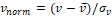 where  is the scaled voxel intensity (in the range of [0, 1]), and  and  are mean and standard deviation of  over all preprocessed scans in the training set. Preprocessing was the same for training, validation and test data.

U-Net

The custom U-Net is composed of an encoder (contracting path) and a decoder (expanding path) (Figure 1a). The encoder learns about the features of segmentation through computing the feature maps at multiple scales based on the training scans [21]. The decoder provides the gradual synthesis of the full-resolution segmentation mask from the low-resolution feature maps by up-sampling [21].
In the encoder, each layer consists of two 3x3 convolutions with padding of 1 (for keeping the dimension of feature maps constant), each followed by batch normalization and a rectified linear unit. Then, downsampling is carried out with 2x2 max pooling with a stride of 2, reducing the resolution of feature maps to half of its original. The number of feature maps is doubled in the subsequent convolution. The most important features are passed to the next layer while the image dimension is halved.
The decoder has the same components as the encoder except that max pooling is replaced by 2-fold up-sampling. After up-sampling, the expanded feature map is zero-padded if necessary and then concatenated with the corresponding feature map from the encoder. Then the feature maps undergo the same processing steps as in the encoder, i.e. two 3x3 convolutions with padding of 1, each followed by batch normalization and a rectified linear unit. The number of feature maps is halved while their dimensions are doubled when they move up a layer along the decoder. At the final step, a 1x1 convolution is used for combining all 64 feature vectors to compute the segmentation on voxel basis. Thus, the output segmentation mask has the same size as the individual MRI.

Training of the U-Net

Training scans were sliced in three orientations (transaxial, sagittal, coronal) resulting in three sets of 2-dimensional image slices (Figure 1b). Within each epoch, the U-Net was trained sequentially with all three sets. Training by one of the sets was executed as follows. Sixteen slices were randomly drawn from the training set. A patch of 128x128 pixels was cropped randomly on each slice, resulting in a batch of 16 patches that served as an input to the U-Net. Batch feeding was repeated until all slices in the set had been used. As the model is trained with 2-dimensional slices of all three orientations, it is denoted as “2.5D CNN-trained model”.
The free parameters of the U-net (n=13,394,177) were optimized using the Adam optimizer [22]. The loss between the target and the network output was measured by the binary cross-entropy loss , where N (=16) is the batch size, and yn and xn are the target (true label) and the output for the n-th patch, respectively.
A learning rate of 5x10-4 was used, and the U-Net was trained for 100 epochs. The models at every 10th epoch were saved and their performance was evaluated in the independent validation set using the Dice coefficient to measure the agreement with the standard-of-truth. The model trained for 50 epochs was selected for further testing.

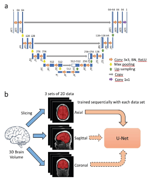
Figure 1: The U-Net architecture is shown in part (a). Blue boxes denote feature maps. The number above the feature map specifies the depth of the feature map wheras its spatial dimension is shown at the bottom of the map. White boxes represent the feature maps concatenated to the decoder. Training of the U-Net is illustrated in part (b).

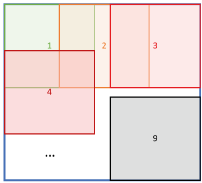
Figure 2: Application of the U-Net to a 2-dimensional image slice. The slice is partitioned into overlapping 128x128 patches, which are fed into the U-Net one by one. The output of the U-net (preliminary TIV segmentation mask) is placed at the exact location of the patch. Pixels are averaged where patches overlap.

Application of the U-Net

For applying the U-net, the preprocessed MR scans are also sliced in three orientations resulting in three sets of 2-dimensional image slices. The TIV segmentation mask is generated slice by slice, separately for each orientation. Nine patches of 128x128 voxels are cropped on each slice (Figure 2). Each patch is fed into the U-Net and the corresponding output is a preliminary segmentation mask of the patch with voxel intensities ranging from 0 (= voxel most likely does not belong to the TIV) to 1 (= voxel most likely belongs to the TIV). The preliminary segmentation mask is placed at the exact location of the patch. When two or more patches overlap, the overlapping voxels are averaged. This results in three different preliminary TIV segmentation masks, one for each orientation of the 2-dimensional slices. These are summed together, then smoothed by a Gaussian filter with a kernel size of 1.5, thresholded at 1.5 (maximum value after addition=3), and lastly resampled to the original resolution of the MR scan using bilinear interpolation for creation of the final binary TIV mask.

Short term test-retest stability and stability across field strengths

Short term test-retest stability and stability across field strengths of TIV estimates were assessed in an independent test set comprising 152 ADNI subjects (“reproducibility test set”). For each subject in the reproducibility test set, a pair of back-to-back T1-weighted scans had been acquired within the same imaging session (without patient repositioning) at both 1.5T and 3T [23-25]. Fifty-one subjects were cognitively normal (CN), 74 had MCI and 27 had Alzheimer’s disease dementia.
The relative absolute difference  was used to quantify the difference between two TIV estimates v1 and v2. To characterize the test-retest stability, v1 and v2 were the TIV estimates from a pair of back-to-back scans. To measure the stability across field strengths, v1 and v2 were the TIV estimates from the (first) scan at 1.5T and from the (first) scan at 3T of the same subject.

Impact on the performance of age- and TIV-corrected hippocampus volume for prediction of dementia in MCI patients

The impact of TIV estimates on the performance of age- and TIV-corrected hippocampus volume (HV) to predict MCI-to-dementia progression was assessed in a second test set, which was comprised of the first baseline T1-weighted MR scans of 198 ADNI MCI patients and 137 ADNI CN subjects who had remained cognitively stable for at least 36 months after their baseline scans (“hippocampus test set”). The eligibility criteria and characteristics of this data set were described previously [26,27]. Forty MCI patients and 40 CN subjects in the hippocampus test set were also included in the reproducibility test set.
Unilateral HV was determined using the FIRST module of the FMRIB Software Library (version 5.0) as described previously [26]. The total HV was obtained as the sum of left and right HV. Hippocampus segmentation failed in 2 subjects (1 MCI, 1 CN) who were excluded from further analyses. The age range of the remaining 136 CN subjects was similar to that of the remaining 197 MCI patients (75.8±5.3y versus 74.8±7.2y, P=.16). Ninety-four MCI patients had converted to AD dementia during an observation period of 36 months (32 after 12 months, 42 between 12 and 24 months, and 20 between 24 and 36 months). The remaining 103 MCI patients had remained cognitively stable over 36 months.
The effect of age and TIV on HV in the CN subjects was assessed by bilinear regression: . The resulting regression model was used to correct HV in MCI subjects for age and TIV according to the following formula: , where  and  are the mean age and mean TIV of the CN subjects respectively. Correction for age and TIV was performed separately for CNN-TIV and SPM-TIV.
The power of age- and TIV-corrected HV to predict dementia in the MCI patients was evaluated with receiver operating characteristic (ROC) analysis, using area (AUC) under the ROC curve as performance measure. Delong’s test was employed to compare the AUC of age- and TIV-corrected HV between CNN-TIV and SPM-TIV. The pROC package was used for ROC analysis.

Difficult clinical cases

TIV segmentation by the U-Net was tested on six ‘difficult’ clinical cases: three patients with resection cavity after epilepsy surgery and three patients with brain tumor.

Results

Short term test-retest stability and stability across field strengths

Scatter plots of CNN-TIV versus SPM-TIV in the reproducibility test set are shown in Figure 3. There were six outliers at 1.5T: three amongst the first scans and three amongst the second scans (an outlier was defined as the residual deviates from linear regression for more than 3 interquartile ranges (IQR), i.e., below (lower quartile–3*IQR) or above (upper quartile +3*IQR)). There were two outliers at 3T: one amongst the first scans and another amongst the second scans. The outlier(s) amongst the first and second scans referred to the same subjects at both field strengths. The outlier at 3T was also an outlier at 1.5T. Visual inspection of the outliers’ TIV segmentation revealed oversegmentation by SPM12 (Figure 4). In the remaining cases of the reproducibility test set (outliers excluded), CNN-TIV and SPM-TIV were very strongly correlated: Pearson’s correlation coefficient=0.978, 0.977, 0.972, and 0.969 for the first and second scans at 1.5T, the first and second scans at 3T (all P<.001). CNN-TIV estimates were larger than SPM-TIV estimates under all conditions: 67±33ml, 67±33ml, 45±37ml, 45±39ml for the first and second scans at 1.5T, and the first and second scans at 3T (all paired t-test P<.001; Table 1).
The RAD of TIV estimates between the first and second scans in the reproducibility test set were smaller for CNN at both field strengths: RAD=2.1±2.8‰ versus 3.1±4.4‰ at 1.5T (paired t-test P=.004), 2.2±2.7‰ versus 2.8±2.7‰ at 3T (paired t-test P=.03; Figure 5). The differences remained statistically significant (P=.01 and P=.03) when the outliers were excluded.
TIV estimates were larger at 1.5T compared to 3T for both U-Net and SPM12: first-scan CNN-TIV difference (1.5T-3T)=32±44ml (P<.001), and first-scan SPM-TIV difference (1.5T-3T)=10±37ml (P=.001) (outliers excluded). The RAD of first-scan TIV estimates between 1.5T and 3T was larger for CNN compared to SPM12: 29.3±22.3‰ versus 20.2±17.2‰ (outliers excluded; paired t-test P<.001).

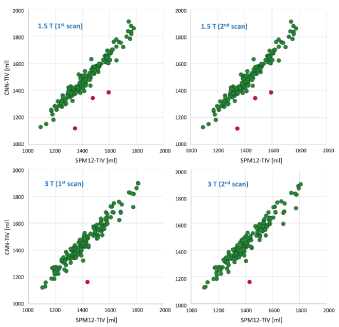
Figure 3: Scatter plots of CNN-TIV versus SPM-TIV in the reproducibility test set. Red dots indicate outliers.

Table 1: TIV estimates by the U-Net (CNN-TIV) and SPM12 (SPM-TIV) in the reproducibility test set.

field strength [T]	category	CNN-TIV (mean±SD) [ml]	SPM-TIV (mean±SD) [ml]
1.5	first scan	1496±159	1434±149
1.5	second scan	1495±159	1433±149
3	first scan	1464±158	1421±152
3	second scan	1463±158	1421±152

Table 2: Area under the ROC curve for prediction of dementia in the hippocampus test set by MRI-based hippocampus volume with correction for age and CNN-TIV, with correction for age and SPM-TIV, and without correction for age and TIV. The 95% confidence interval is given in square brackets. The area under the ROC curve did not differ between any pair of correction methods for any follow-up period (all DeLong test P≥0.21).

	within 12 months (32 progressors)	within 24 months (74 progressors)	within 36 months (94 progressors)
correction for age and CNN-TIV	0.772 [0.685–0.859]	0.688 [0.609–0.767]	0.691 [0.616–0.765]
correction for age and SPM-TIV	0.774 [0.687–0.860]	0.691 [0.612–0.770]	0.693 [0.619–0.767]
no correction for age and TIV	0.762 [0.665–0.860]	0.663 [0.579–0.747]	0.677 [0.601–0.753]

Impact on the performance of age- and TIV-corrected hippocampus volume for prediction of dementia in MCI patients

The scatter plot of CNN-TIV versus SPM-TIV in the hippocampus test set is shown in Figure 6. There were five outliers, 3 MCI patients and 2 CN subjects. The 2 CN outliers were also outliers in the reproducibility test set, but the 3 MCI outliers were not. Visual inspection of the TIV segmentation revealed over segmentation by SPM12 in all three MCI outliers (Figure 7). In the remaining cases (outliers excluded), CNN-TIV and SPM-TIV were strongly correlated: Pearson’s correlation coefficient=0.981 (P<.001). CNN-TIV estimates were 64±29ml larger than SPM-TIV estimates (outliers excluded; paired t-test P<.001).
Bilinear regression of HV in the ADNI CN subjects (except the two outliers) with age and CNN-TIV as independent variables estimated the regression coefficients =-4.954*10-2ml/y and =2.040*10-3ml/ml (=75.9y, CNN-=1499ml). When age and SPM-TIV were used as independent variables in the bilinear regression of HV, the regression coefficients were =-4.800*10-2ml/y and =2.001*10-3ml/ml (SPM-=1433ml). Bilinear regression with age and CNN-TIV explained 18.6% of the HV variance in the CN subjects, while bilinear regression with age and SPM-TIV explained 17.1% of the variance.
The power of age- and TIV-corrected hippocampus volume for prediction of dementia in the MCI patients of the hippocampus test set as measured by the AUC did not differ between CNN-TIV and SPM-TIV (all DeLong test P≥.21; Table 2).
Finally, age- and TIV-corrected HV estimates were transformed to z-scores using the formula , where is the corrected HV in the individual subject, and  and  are the mean and standard deviation of the corrected HV in the ADNI CN subjects (without outliers) respectively. Transformation to z-scores was performed separately for CNN-TIV and SPM-TIV. In the five outliers, z-scores with CNN-TIV were larger than with SPM-TIV (Figure 6). The z-score difference of the outliers ranged between 0.32 and 0.68. For comparison, the z-score of the stable MCI patients was on average 0.72 larger than the z-score of the MCI patients who progressed to dementia within 3 years (outliers excluded).

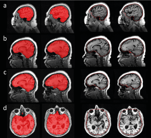
Figure 4: Outliers in the comparison of CNN-TIV (left columns) versus SPM-TIV (right columns) in the reproducibility test set: (a) ADNI subject 002_S_1280 at 1.5T, (b) 052_S_1250 at 1.5 T, (c) 052_S_1250 at 3 T, (d) 133_S_0629 at 1.5T. Displayed images are the TIV segmentations of the first scans in the session, the segmentation results for the second scans were very similar.

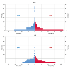
Figure 5: Histograms of the relative absolute difference (RAD) of TIV estimates between first and second scan in the same imaging session at the field strengths of 1.5T (top) and 3T (bottom) in the reproducibility test set, comparing the test-retest stability between SPM-TIV (left) and CNN-TIV (right).

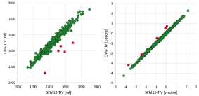
Figure 6: Scatter plots of CNN-TIV versus SPM-TIV in volume [ml] (left) or as z-score (right) in the hippocampus test set. Red dots indicate outliers.

Difficult clinical cases

TIV segmentation by the U-Net worked properly in all difficult clinical cases, all lesions were included in the TIV mask (Figure 8).

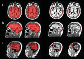
Figure 7: Outliers in the comparison of CNN-TIV (left columns) versus SPM-TIV (right columns) in the hippocampus test set: (a) ADNI subject 023_S_0042, (b) 036_S_0976, (c) 109_S_0950.

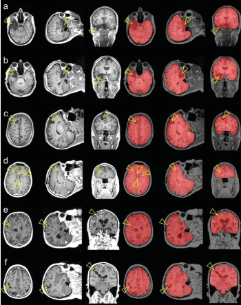
Figure 8: TIV segmentation by the U-Net in six ‘difficult’ cases, three patients with resection cavity after epilepsy surgery (a-c) and three patients with brain tumor (d-f). The arrow heads point to the lesions.

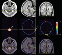
Figure 9: The middle row shows a transaxial (left), coronal (middle), and sagittal (right) slice of the mean difference between CNN-TIV and SPM-TIV estimated from the 1.5T scans in the reproducibility test set (first and second scans) in MNI space. The individual spatial normalisation transformations estimated by SPM12 during SPM12 TIV segmentation were used to transform individual difference images from patient space to MNI space. The lower row shows the mean difference between the TIVs overlaid to the MR scan of a single subject, while the MRI in MNI space is shown at the top row. The mean difference was close to 1 in lower parts of brainstem (yellow arrows) and in blood filled sinuses (red arrow), indicating that these regions were systematically included by the U-Net TIV segmentation, but excluded in SPM12 TIV segmentation.

Discussion

U-Net TIV estimates were very strongly correlated with SPM12 TIV estimates in both test sets. This demonstrates the usefulness of the U-Net approach for automatic TIV estimation, as SPM12 is generally considered a particularly effective method for automatic TIV estimation [14].
The present findings suggest the U-Net to be even slightly superior to SPM12. First, SPM12 resulted in TIV over segmentation in up to 2.0% of the cases. Second, test-retest stability of TIV estimates in back-to-back scans of the reproducibility test set was better with the U-Net than with SPM12. U-Net computation time (including preprocessing) of 2 minutes in TIV segmentation on a standard PC makes it fit for daily clinical practice (SPM12: 10 minutes).
TIV estimates in the reproducibility test set were larger at 1.5T compared to 3T for both U-Net and SPM12, but the U-Net was more sensitive to the field strength (average 1.5T–3T difference of 32ml versus 10ml for U-Net and SPM12). Probably it is because the training set was imbalanced with respect to field strength (1.5T:3T=2.92:1). We hypothesize that the U-Net can be trained to be less sensitive to varying field strength by using manual TIV delineation as gold-standard in a balanced training set in terms of field strength and/or using the field strength as an additional input parameter to the network.
CNN-TIV was on average about 50ml larger than SPM12-TIV. The U-Net included more inferior parts of the brain stem as well as the blood filled sinuses, in contrast to SPM12 (Figure 9). This is in line with the findings of Malone and co-workers who reported SPM12-TIV to be on average 40ml smaller than manual TIV estimates, probably due to exclusion of blood-filled sinuses by SPM12 [14]. This suggests that the CNN-TIV estimates might be closer to manual TIV segmentation than SPM12-TIV.
The use of CNN-TIV versus SPM12-TIV for adjusting hippocampus volume with respect to age and TIV showed no impact on the performance of adjusted hippocampus volume to predict dementia in the MCI patients of the hippocampus test set. This might be explained by the fact that reducing the measurement error of hippocampus volume in general has only little impact on its prediction performance, possibly due to a ceiling effect caused by inherent limitations of the predictive power of hippocampal atrophy [28]. However, for a small fraction of patients (the outliers), the difference between CNN-TIV and SPM12-TIV might impact the prediction of future cognitive performance based on age and TIV-adjusted hippocampus volume, as the difference in z-scores of CNN-TIV versus SPM12-TIV can be similar to the mean difference between MCI patients who progress to dementia and MCI patients who remain cognitively stable (Figure 6).
Stability of TIV segmentation by the U-Net was further confirmed in ‘difficult’ clinical cases with brain tumors or resection cavities, where traditional skull stripping methods often have difficulties.
The major limitation of this study was the lack of manual TIV delineation as standard-of-truth for training the U-Net. Still, semi-automatically generated SPM12-TIV is considered a particularly effective substitute for manual TIV [14]. Furthermore, the use of SPM12-TIV for U-Net training is expected to cause a bias in favor of SPM12 in the comparison of U-Net and SPM12 performance in the independent ADNI samples. We hypothesize that U-Net training with TIV delineated manually as standard-of-truth would result in a more pronounced performance benefit of the U-Net compared to SPM12.

Conclusion

In conclusion, the findings of this study support the use of a U-Net trained with good SPM12-TIV segmentation for automatic TIV estimation in settings with uniform field strength, including assessment of individual patients in routine patient care. Further improvement, including improved stability with respect to the field strength, might be achieved by training the U-Net with manual expert TIV delineation in a training set balanced for field strengths.

Acknowledgments

Data collection and sharing of ADNI datasets was funded by the Alzheimer's Disease Neuroimaging Initiative (ADNI) (National Institutes of Health Grant U01 AG024904) and DOD ADNI (Department of Defense award number W81XWH-12-2-0012). ADNI is funded by the National Institute on Aging, the National Institute of Biomedical Imaging and Bioengineering, and through generous contributions from the following: AbbVie, Alzheimer’s Association; Alzheimer’s Drug Discovery Foundation; Araclon Biotech; BioClinica, Inc.; Biogen; Bristol-Myers Squibb Company; CereSpir, Inc.; Cogstate; Eisai Inc.; Elan Pharmaceuticals, Inc.; Eli Lilly and Company; EuroImmun; F. Hoffmann-La Roche Ltd and its affiliated company Genentech, Inc.; Fujirebio; GE Healthcare; IXICO Ltd.; Janssen Alzheimer Immunotherapy Research & Development, LLC.; Johnson & Johnson Pharmaceutical Research & Development LLC.; Lumosity; Lundbeck; Merck & Co., Inc.; Meso Scale Diagnostics, LLC.; NeuroRx Research; Neurotrack Technologies; Novartis Pharmaceuticals Corporation; Pfizer Inc.; Piramal Imaging; Servier; Takeda Pharmaceutical Company; and Transition Therapeutics. The Canadian Institutes of Health Research is providing funds to support ADNI clinical sites in Canada. Private sector contributions are facilitated by the Foundation for the National Institutes of Health (www.fnih.org). The grantee organization is the Northern California Institute for Research and Education, and the study is coordinated by the Alzheimer’s Therapeutic Research Institute at the University of Southern California. ADNI data are disseminated by the Laboratory for Neuro Imaging at the University of Southern California.

Grant support

This study was supported by the Federal Ministry for Economic Affairs and Energy of Germany (ZIM ZF4446501AW7, ZF4268402AW7).

Acknowledgements and Disclosure

Conflict of interest disclosure statement

JK, A-CO, LS, and RO are full-time employees of jung diagnostics GmbH. PS is full-time employee of Olympus Surgical Technologies Europe. The other authors do not have potential conflicts of interest concerning this manuscript.

References

1. Giorgio A, De Stefano N (2013) Clinical use of brain volumetry. J Magn Reson Imaging 37: 1-14. [Crossref]
2. Barnes J, Ridgway GR, Bartlett J, M D Henley S, Lehmann M, et al. (2010) Head size, age and gender adjustment in MRI studies: a necessary nuisance? Neuroimage 53: 1244-1255. [Crossref]
3. Westman E, Aguilar C, Muehlboeck JS, Simmons A (2013) Regional Magnetic Resonance Imaging Measures for Multivariate Analysis in Alzheimer's Disease and Mild Cognitive Impairment. Brain Topogr 26: 9-23. [Crossref]
4. Walhovd KB, Fjell AM, Reinvang I, Lundervold A, Dale AM, et al. (2005) Effects of age on volumes of cortex, white matter and subcortical structures. Neurobiol Aging 26: 1261-1270. [Crossref]
5. Mathalon DH, Sullivan EV, Rawles JM, Pfefferbaum A (1993) Correction for head size in brain-imaging measurements. Psychiatry Res 50: 121-139. [Crossref]
6. Ikram MA, Fornage M, Smith AV, Seshadri S, Schmidt R, et al. (2012) Common variants at 6q22 and 17q21 are associated with intracranial volume. Nat Genet 44: 539-544. [Crossref]
7. Sargolzaei S, Sargolzaei A, Cabrerizo M, Chen G, Goryawala M, et al. (2015) A practical guideline for intracranial volume estimation in patients with Alzheimer's disease. BMC Bioinformatics 16Suppl 7: S8. [Crossref]
8. Arndt S, Cohen G, Alliger RJ, Swayze VW, 2nd, Andreasen NC (1991) Problems with ratio and proportion measures of imaged cerebral structures. Psychiatry Res 40: 79-89. [Crossref]
9. Nordenskjold R, Malmberg F, Larsson EM, Simmons A, Brooks SJ, et al. (2013) Intracranial volume estimated with commonly used methods could introduce bias in studies including brain volume measurements. Neuroimage 83: 355-360. [Crossref]
10. Hansen TI, Brezova V, Eikenes L, Haberg A, Vangberg TR (2015) How Does the Accuracy of Intracranial Volume Measurements Affect Normalized Brain Volumes? Sample Size Estimates Based on 966 Subjects from the HUNT MRI Cohort. Am J Neuroradiol 36: 1450-1456. [Crossref]
11. Perneczky R, Wagenpfeil S, Lunetta KL, Cupples LA, Green RC, et al. (2010) Head circumference, atrophy, and cognition: implications for brain reserve in Alzheimer disease. Neurology 75: 137-142. [Crossref]
12. Whitwell JL, Crum WR, Watt HC, Fox NC (2001) Normalization of cerebral volumes by use of intracranial volume: implications for longitudinal quantitative MR imaging. AJNR Am J Neuroradiol 22: 1483-1489. [Crossref]
13. Eritaia J, Wood SJ, Stuart GW, Bridle N, Dudgeon P, et al. (2000) An optimized method for estimating intracranial volume from magnetic resonance images. Magn Reson Med 44: 973-977. [Crossref]
14. Malone IB, Leung KK, Clegg S, Barnes J, Whitwell JL, et al. (2015) Accurate automatic estimation of total intracranial volume: a nuisance variable with less nuisance. Neuroimage 104: 366-372. [Crossref]
15. Dale AM, Fischl B, Sereno MI (1999) Cortical surface-based analysis. I. Segmentation and surface reconstruction. Neuroimage 9: 179-194. [Crossref]
16. Ashburner J, Friston KJ (2005) Unified segmentation. Neuroimage 26: 839-851. [Crossref]
17. Weiskopf N, Lutti A, Helms G, Novak M, Ashburner J, et al. (2011) Unified segmentation based correction of R1 brain maps for RF transmit field inhomogeneities (UNICORT). Neuroimage 54: 2116-2124. [Crossref]
18. LeCun Y, Bengio Y, Hinton G (2015) Deep learning. Nature 521: 436-444. [Crossref]
19. Litjens G, Kooi T, Bejnordi BE, Adiyoso Setio AA, Ciompi F, et al. (2017) A survey on deep learning in medical image analysis. Med Image Anal 42: 60-88. [Crossref]
20. Keihaninejad S, Heckemann RA, Fagiolo G, Symms MR, Hajnal JV, et al. (2010) A robust method to estimate the intracranial volume across MRI field strengths (1.5T and 3T). Neuroimage 50: 1427-1437. [Crossref]
21. Falk T, Mai D, Bensch R, Çiçek O, Abdulkadir A, et al. (2019) U-Net: deep learning for cell counting, detection, and morphometry. Nat Methods 16: 67-70. [Crossref]
22. Kingma DP, Ba JL (2017) ADAM: A method for stochastic optimization.
23. Jack CR, Bernstein MA, Fox NC, et al. The Alzheimer's Disease Neuroimaging Initiative (ADNI): MRI methods. J Magn Reson Imaging. 2008;27:685-91. [Crossref]
24. Cavedo E, Suppa P, Lange C, Thompson P, Alexander G, et al. (2017) Fully Automatic MRI-Based Hippocampus Volumetry Using FSL-FIRST: Intra-Scanner Test-Retest Stability, Inter-Field Strength Variability, and Performance as Enrichment Biomarker for Clinical Trials Using Prodromal Target Populations at Risk for Alzheimer's Disease. J Alzheimers Dis 60: 151-164. [Crossref]
25. Wolz R, Schwarz AJ, Yu P, Cole PE, Rueckert D, et al. (2014) Robustness of automated hippocampal volumetry across magnetic resonance field strengths and repeat images. Alzheimers Dement 10: 430-438. [Crossref]
26. Suppa P, Hampel H, Kepp T, Lange C, Spies L, et al. (2016) Performance of Hippocampus Volumetry with FSL-FIRST for Prediction of Alzheimer's Disease Dementia in at Risk Subjects with Amnestic Mild Cognitive Impairment. J Alzheimers Dis 51: 867-873. [Crossref]
27. Suppa P, Hampel H, Spies L, Fiebach JB, Dubois B, et al. (2015) Fully Automated Atlas-Based Hippocampus Volumetry for Clinical Routine: Validation in Subjects with Mild Cognitive Impairment from the ADNI Cohort. J Alzheimers Dis 46: 199-209. [Crossref]
28. Buchert R, Lange C, Suppa P, Apostolova I, Spies L, et al. (2018) Magnetic resonance imaging-based hippocampus volume for prediction of dementia in mild cognitive impairment: Why does the measurement method matter so little? Alzheimers Dement 14: 976-978. [Crossref]