Take a look at the Recent articles

Abstract

This paper describes how ERP energy density analysis and marginal cost-benefit analysis were combined to interpret the results of an investigation of mental performance. Eleven subjects competed in performing computer-generated mental arithmetic tasks over a period lasting, in some cases, 2.5 hours. Assuming that brain resources are dynamically allocated, marginal cost-benefit analysis of optimal resource allocation was used to interpret longitudinal changes in these subjects' ERP energy density. It was possible to graphically track each subject through four phases: learning, boredom, motivation, and fatigue. Phase trajectories of this sort may be useful in rehabilitation therapy as well as human factors research.

Key words

vent Related Potentials, Electroencephalography, EEG, Cognitive Fatigue, Mental Workload, Brain Resource Allocation

Introduction

This paper describes the results of a small pilot level project that demonstrated the use of EEG (electroencephalography) to monitor cognitive performance. The project involved just a few volunteers but focuses upon the possible future development of the procedure to monitor cognitive improvement and fatigue of brain injured or cognitively impaired patients or other individuals who perform complex cognitive tasks over an extended period. We believe that the procedure described here may also have potential value in some forms of clinical research and assessment of the benefits of physical therapy. Our focus is entirely on the procedure; no hypotheses regarding cognitive neurophysiology are implied or tested. And all references are to widely accepted sources of particular experimental or mathematical steps of this procedure.

If one assumes that the brain strives (automatically or under volitional control) to achieve maximum efficiency in allocation of limited processing resources, then it is appropriate to exploit the theory of optimal resource allocation in monitoring aspects of brain function. As Rosen [1] emphasizes, optimality principles are widely applicable in the biological sciences. Section 1 of this paper reviews the key features of resource allocation theory and points out several ways in which it provides insight for the analysis of human cognitive performance. Section 2 demonstrates the value of this theoretical insight by applying it to EEG data.

Optimal brain resource allocation

A foundation concept in the study of optimal resource allocation is the comparison of the extra (or “marginal”) benefits of allocating more resources to some particular activity, versus the extra (or “marginal”) opportunity costs. The latter are assessed by considering the benefits that are sacrificed as the resources are taken from some alternative activity. This applies not only to explicit human decisions but is presumed to explain many biological processes as well.

For example, the famous economist, Milton Friedman [2] has emphasized the broader nature of economic theory by citing the growth of a tree limb as an example of optimal resource allocation. As a tree limb grows it expands the tree’s leaf area and its photosynthetic access to solar energy. But at some point, the extra energy obtained is exhausted by the extra energy required to grow and maintain the limb. It obviously would be a poor allocation of the tree’s resources to grow limbs beyond this point.

This point of view is applied here as two basic assumptions: The first is that the brain does attempt to optimally allocate limited resources among several concurrent activities. The manner in which the brain does this need not be specified. The second necessary assumption is that every possible beneficial brain activity adds less and less to the individual’s welfare as it is pursued more and more extensively. The incremental gains are smaller and smaller --- until they are simply not worth the effort. This is the universal “law of diminishing marginal utility”. It is, mathematically, an assumption that the first partial derivative of welfare or benefit with respect to the level of the activity is downward sloping. For present purposes one need not know the degree of slope, other than that it is negative [3].

Graphical depiction of the theory

Figure 1 illustrates a marginal benefit function (MB). The horizontal axis shows the level of performance of some activity. (Let us call it activity A.) The vertical axis shows the extra benefit associated with each value on the horizontal axis. Since it would be irrational to "pay" more for anything than the extra benefit of having it, the vertical axis also shows the amount of brain resources that would be allocated to (expended upon) the given activity. Thus, the downward slope of the marginal benefit function shows that it is "worth" less and less to the individual (in terms of resource expenditure) to move to each higher level of performance.

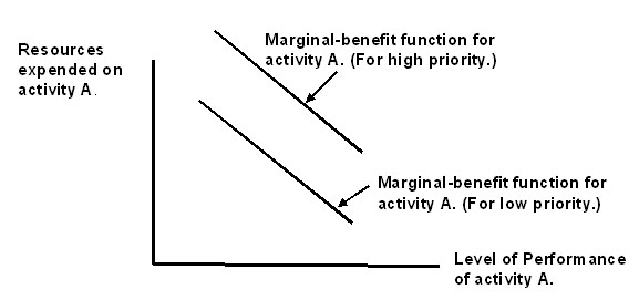
Figure 1. Marginal benefit function (MB).

Also, two possible locations of the marginal benefit curve are shown in Figure 1, illustrating that if the given activity suddenly acquires a higher priority, the whole marginal benefit curve would shift upward. Such an upward shift in a marginal benefit curve is what we usually mean by increased "motivation." The activity has, for some reason, acquired greater significance to the individual, and any given level of performance is worth more resource expenditure than before.

Figure 2 shows a marginal cost function (MC) for activity A, which is just the marginal benefit sacrificed by pursuing that activity at the expense of other brain activities. Its upward slope reflects the downward slope of those other MB functions, since a higher level of performance of activity A would imply moving leftward along the horizontal axes of their marginal benefit functions. Figure 2 also shows the effect of those other activities becoming more significant to the individual: The marginal cost curve for activity A would shift upward, since every level of activity A would then entail a higher marginal opportunity cost than before.

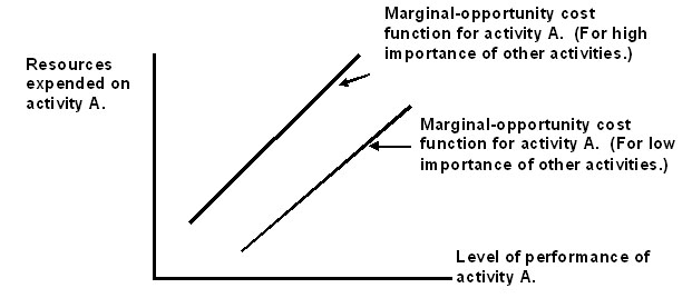
Figure 2. Marginal cost function (MC).

An example of applying the marginal cost-benefit analysis:

An upward shift in a marginal cost curve is, we believe, the most useful way to abstractly characterize “cognitive fatigue.” As a brain devotes more and more resources to a primary cognitive task, other brain activities must be denied those resources. Over time, or as the situation becomes more stressful, the opportunity cost will increase. Postponed system maintenance tasks will begin to become more urgent. Simple examples are the need to rest, or stretch, or go to the bathroom. A vast number of other activities, connected with perception, memory updating, maintenance of affective tone, and physiological homeostasis may also be partly postponed in order to concentrate attentional and other resources on the primary task. But the growing urgency of attending to any or all of these postponed activities will eventually shift the marginal opportunity cost function for the primary task upward. Any given level of performance of activity A will cost more than before.

As Hockey [4], and others have described, the brain tries to reorganize the performance of a primary task in order to reduce its demand upon brain resources. A balance is achieved when each activity is pursued to the level that equates its marginal benefit with its marginal cost. This occurs at the intersection of the marginal benefit and marginal cost curves, as shown in Figure 3.

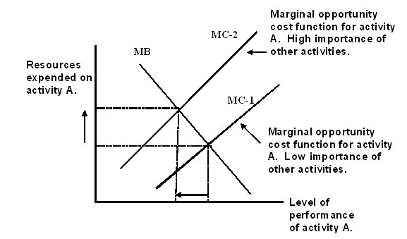
Figure 3. Intersection of the marginal benefit and marginal cost curves.

A shift (upward or downward) in either function, MB or MC, will of course require a rebalancing. A shift of either curve in Figure 3 will move the intersection along the curve that has not shifted. Although this is geometrically obvious, it is the most important feature of the analysis. For it allows us to relate changes in the level of resource allocation to the task, and changes in performance, to shifts in the curves which may be mapped to such constructs as "motivation" and "cognitive fatigue."

In Figure 3 we have illustrated, for example, the effect of cognitive fatigue. As the growing urgency of other tasks shifts the MC curve upward from MC-1 to MC-2, the brain's resources must be reallocated to keep marginal cost equal to marginal benefit. For activity A, this reallocation is shown by the movement of the intersection upward to the left along the MB curve. At first, this may seem counter-intuitive. The growing urgency of activity B, C, etc., leads, surprisingly, to an increase in resources expended on A. This result is easy to understand, however, if the movement is viewed in two steps: First, the urgency of other activities) shifts upward the whole marginal opportunity cost function for activity A. But assuming no change in the importance of activity A itself, relative to various levels of performance, it becomes necessary to expend even more resources to that activity. As, Hockey [4] and others have described, the brain tries to reorganize the performance of a primary task in order to reduce its demand upon brain resources.

In some cases, this pattern of reallocation of resources may lead to catastrophe. As an example (one that is more physical than cognitive), picture a small boy in a play-ground, hanging by his hands from the crossbar of a jungle gym. As the child reaches the limit of his endurance, he will likely start to squirm, improve his grip, even grimace, as if that would help. What we see is an increase in energy devoted to the task. The metabolic cost of performing the activity has increased because tired muscles can no longer be starved of oxygen. Yet the prospect of falling increases the marginal value of hanging on, and hence justifies an even greater energy commitment. As this is a self-reinforcing (positive feedback) loop, the challenge worsens until the child gives up and drops to the ground. With regard to mental activities it seems that the final outcome of the pattern described above is best called “mental exhaustion” rather than merely “cognitive fatigue.”

Geometric clarification of terms

The marginal cost-benefit analysis shows that certain combinations of the variables represent points on the same continuum (along one of the curves) while other combinations reflect movement of a curve and its intersection with the other one.

For example, “fatigue” would shift the marginal cost function upward as shown in Figure 3. Its intersection with the marginal benefit function would slide upward to the right, leading to a decrease in performance of the primary task at the same time that more resources are committed to the task. It is important to note that these are in opposite directions. This opposition would also be the result of a downward shift of the marginal cost curve. This would depict the result of skill development including development of automated responses to a challenge, which would increase performance and decrease resource use. For our purposes we shall label it “learning.”

Figure 3 shows that there is only one way in which performance and resource commitment to a task can change in the same direction. This can only happen if the marginal benefit curve shifts. For example, a downward shift would depict the task being regarded as less important; and the result would be a decrease in both performance and resource commitment. For convenience we shall label this “boredom,” – and a shift of the marginal benefit curve in the other direction (outward) seems appropriately labeled “motivation.” The latter would result in a greater commitment of resources and an increase in performance.

Summary of the logic

This marginal cost-marginal benefit analysis will provide a framework for interpreting the data described in the next section. There it will be explained that EEG recordings can be transformed to measure the intensity of brain resources committed to an experimental task. When combined with task performance data, there are only four possible outcomes, and these can be interpreted as follows:

• If both resource commitment and performance are increasing, then the MB curve is shifting upward (increased motivation).
• If both resource commitment and performance of an activity are decreasing, the MB curve is shifting downward (decreased motivation or boredom).
• If performance of an activity increases while fewer resources are committed to it, then the MC curve is shifting downward (learning).
• If performance of an activity decreases while more resources are committed to it, then the MC curve is shifting upward (fatigue).

EEG Demonstration

This section reports how topographic EEG recordings were transformed into energy density ERPs for the current project. It assumes some familiarity with EEG data collection, especially collection of Event-related-potentials (ERPs). Specific details as to the derivation of the energy density ERPs used in this paper and additional applications can be found in a “Primer” that is posted on the Research Gate” website as a working paper [5].

ERPs allow us to “average-out” brain activity not related to the task [6]. Then, with modern multi-channel ERPs it is a simple matter to calculate the level of scalp energy density reflected in each ERP [7]. Although most of the energy used in brain activity is dissipated in the form of heat, carried away in the brain blood flow [8], some part is dissipated as the energy that maintains the scalp electrical fields that are sensed by EEG. We assume therefore that the average energy density of an ERP is proportional to the extent of brain activation committed to the gating task. (This is similar to the assumed linkage between brain activation and uptake of radioactive tracers that underlies brain scanning techniques like PET). On this basis, we hypothesized that rising levels of scalp energy density would be seen in ERPs taken, say, every 15 minutes, as a subject repetitively performed a complex cognitive task (mental arithmetic in this case) -- especially as the subject reached the stage where performance rapidly deteriorated and the subject became too exhausted to continue. Before that stage, we also expected to see occasions of over-compensation, i.e., "learning," or other states as summarized above in Section 1.

Method

Eleven subjects, college-educated, ages 20 through 35, all of them colleagues at NASA’s Ames Research Laboratory, volunteered to compete in performing a computer-generated mental arithmetic task, repetitively for as long as possible, while instrumented for EEG. Though unpaid and unrewarded, each volunteer was eager to “win” by excelling at both accuracy and endurance. Their scores were posted as they finished.

The task consisted of calculating the algebraic sum of four one-digit numbers presented in the center of a computer screen. For example, 6 - 2 + 9 - 3. The numbers were random generated but were filtered to prevent obvious sums (such as 1 - 1 - 2 + 2) and an “answer” was presented which was, at random, often incorrect (75%), but close. The subject was required to determine if the algebraic sum was higher than, equal to, or lower than the proposed “answer,” and indicate the decision by pressing one of three keys on a special hand-held keypad. Each response triggered presentation of a new problem after a five-second delay. Response times and number of errors were recorded automatically but were not revealed to the subject until the end of the session.

A 21-channel EEG recording was made while the subject performed the task, using a Lexicor NRS-24 system (Boulder, CO) with 3200x analog gain, 0.5 Hz high-pass filter, 60 Hz notch filter, and maximum scalp impedance of 5000 ohms. The analog signal was digitized at 256 samples per second. Scalp electrodes were applied according to the International Standard 10-20 pattern [9,10], using the Physometric, Inc. eNET electrode cap (Billercia, MA) and EEG-Sol electrode paste (part number 16-004, Meditrace Products Division of Graphic Controls, Inc., Buffalo, NY).

Each response by the subject generated a marker in the continuous EEG recording that was later used to identify 600 millisecond stimulus-gated epochs. Those generated during each 15-minute period deemed to be artifact free by visual inspection were then averaged to produce ERPs. Depending upon the subject’s reaction time and the number of epochs that were rejected because of artifacts, the number of epochs generated during a 15-minute varied but was in no case less than 30.

Each 21-channel ERP was mathematically converted to a measure of average scalp energy density (averaged over the 600 msec post-stimulus period and over the 21 electrode sites). This procedure involved fitting a least-squares model equation, V=(a+bX+cY+eXY)^3, expanded as a polynomial, to the grid of 21 voltage values at each time data point, and then using the fitted equation to calculate the second partial spatial derivatives of the implied voltage surface in each coordinate direction. These are components of the Laplacian, which is proportional to scalp charge density [11,12]. Comparison of the fitted voltage surface with the original voltage values produced an R-square value of 0.95 or greater for every data point in each ERP. The product of the estimated charge density and the estimated voltage at each electrode site (and instant in the ERP) is then proportional to scalp energy density at that site, at that instant [13-15]. We assume that energy density, averaged over all scalp electrodes and over the period of the ERP is, in turn, proportional to the brain activity devoted to the gating task (whether diffused or localized).

Results

Some subjects lasted longer than others. One quit after only 45 minutes (long enough for 3 ERPs). Two lasted for 150 minutes (2.5 hours: 10 ERPs). In each case it was the subject who decided to quit. All indicated they were too exhausted to continue. At this point most were visibly exhausted (sweaty, agitated, and anxious to get up and walk around).

Figure 4 & 5 illustrate how the MB-MC analysis can be used to track individual subjects' trajectory through the four possible states: Learning, Motivation, Fatigue, and Boredom.

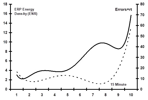
Figure 4. ERP energy density (ENR, solid line, left axis) and errors + rt (dashed line, right axis). Curves shown are polynomial regression lines fit to the data. R-sq. = 0.921 for ENR; 0.927 for errors + rt.

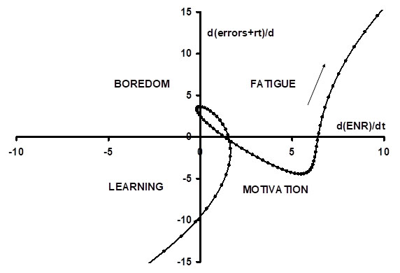
Figure 5. State diagram derived from Figure 4. Data points shown every 1.5 minutes.

These figures pertain to one typical subject. Figure 4 shows the subject’s ERP energy density levels compared to a "performance index". The performance index is simply the unweighted sum of the subject's average reaction time and number of errors during the period of each ERP. Note that the higher the value of this index, the worse the subject's performance; this is a leftward movement along the horizontal axis of figures like Figure 3.

The following table summarizes the logic behind the trajectory (Table 1). It is the same as the summary at the end of Part 1, except that it makes clear that Figure 4 & 5 are based on an index of "bad" performance (rt + errors), which is a leftward movement in figures like Figure 3.

Table 1. Summarizing the logic behind the trajectory.

energy	rt+errors	performance	Curve Shift	Interpretation
up	down	up	MB up	motivation
up	up	down	MC up	fatigue
down	up	down	MB down	boredom
down	down	up	MC down	learning

Discussion

The subject whose state trajectory is shown in Figure 5 was highly typical. Similar to most of the 11 subjects, he started by mainly learning the task, building skill through practice. That is, his performance improved (falling rt + errors) while energy committed to the task also fell. Soon he further improved performance by committing added energy to the task, i.e., the improvement in performance through practice was followed by a further improvement in performance through higher motivation. But then he began to tire: the marginal opportunity cost of performing the task began to rise, as shown by a concurrent increase in (bad) performance (errors + rt) and a decrease in energy. However, as with most subjects, this early period of fatigue was soon followed by a revival of performance through an increased energy commitment (higher motivation) --- until finally he was overcome by uncompensated cognitive fatigue, which we have labeled mental exhaustion. Not all subjects followed this general trajectory, of course. Two started in the "Motivated" quadrant, moved almost immediately into the "Fatigue" quadrant, and quit.

Although the statistical analysis of group averages revealed a "statistically significant" trend -- rising fatigue (i.e., rising energy accompanied by falling performance) -- what may be more important for further research is the possibility of quantifying individuals' detailed state trajectories. Difference and similarities among subjects may be just as important as the general trend toward mental exhaustion (which, after all, is not a surprising trend).

State trajectory analysis applied to individual subjects in a human performance experiment may prove to be a valuable diagnostic tool. It could be combined with the scheduled introduction of special experimental treatments. For example, stress factors such as increases in ambient noise levels or temperature could be introduced at certain points during the experiment.

In addition to potential applications in physical medicine and rehabilitation, we expect applications in human factors engineering experiments. The trajectory analysis could be employed for instance, in the comparison of instrument panel layouts and data displays, mission profile designs, training procedures, and crew selection criteria [16-27].

Conclusions

The procedure described addresses a serious problem in the interpretation of human performance. It is notoriously difficult to determine whether someone's poor performance is evidence of lack of motivation, or lack of resources (capacity to perform). This is a problem that plagues teachers and parents, coaches, and therapists.

The procedure described herein may be used to derive on-line in real time measures of cognitive performance using inexpensive small bedside type monitors. In this way the use of expensive MRI, BOLD and PET facilities can be avoided. The analytical and discriminatory steps in interpreting ERP results are straight forward and can easily be implemented on any laptop computer. As such, it avoids the necessity of complex ERP component analysis.

By combing ERP energy 2021 Copyright OAT. All rights reservst-benefit analysis of brain resource allocation, it is possible to distinguish not only between fatigue and motivational changes, but also between these states and boredom and learning or skill development. We have demonstrated how this analysis can be used to produce a graphical display of a subject's trajectory through a state-space consisting of those four states.

Acknowledgements

This study was, in part, funded through the NASA Ames Research Center Director’s Discretionary Fund for FY 1999/2000 and, in part, as one element in the Psychological and Physiological Stressors and Factors (PPSF) project of NASA's Aerospace Operations Systems Program. The authors wish to thank Ms. Bernadette Luna and Drs. Mark Kliss of NASA Ames Research Center for their help and encouragement during the performance of this investigation.

References

1. Rosen Robert (1967) Optimality Principles in Biology. New York: Plenum Press.
2. Friedman Milton (1953) Essays in Positive Economics. Chicago: University of Chicago Press, 19.
3. Wilde D, Beightler C (1967) Foundations of Optimization. Englewood Cliffs, NJ. Prentice-Hall.
4. Hockey GR (1997) Compensatory control in the regulation of human performance under stress and high workload: A cognitive-energetic framework. Biol Psychol 45: 73-93. [Crossref]
5. Montgomery RW, Montgomery LD, Guisado R (2017) Using scalp electrostatic energy density to study cognition: A step-by-step primer with examples and applications.
6. Vaughan Jr HG (1974) The analysis of scalp recorded brain potentials, Chapter 4 in Thompson, R F. & Patterson, M. M., Biolectric Recording Techniques New York: Academic Press.
7. Montgomery RW, Montgomery LD, Guisado R (1993) Electroencephalographic scalp-energy analysis as a tool for investigation of cognitive performance. Biomed Instrum Technol 27: 137-142. [Crossref]
8. Vasilescu V, Margineanu DG (1982) Introduction to Neurobiophysics, Kent, England: Abacus Press 121-141.
9. Jasper HH (1958) Report of the committee on methods of clinical examination in electroencephalography. Electroenceph Clin Neurophysiol 10: 370-375.
10. Homan R (1988) The 10-20 system and cerebral location. Am J EEG Tech 28: 269-279.
11. Hjorth B (1980) Source derivation simplifies EEG interpretation. Am J EEG Tech 20: 121-32.
12. Nunez PL (1989) Estimation of large scale neocortical source activity with EEG surface Laplacians. Brain Topogr 2: 141-154. [Crossref]
13. Thompson William (1848) Note on the integration of the equations of equilibrium of an elastic solid. Cambrid Dublin Math J 3: 87-89.
14. Feynman R, Leighton R, Sands M (1970) The Feynman Lectures on Physics. Reading, MA.: Addison-Wesley, II-8-10.
15. Lorrain P, Corson D (1962) Electromagnetic Fields and Waves. Freeman & Co. 77.
16. Broadbent DE (1979) Is a fatigue test now possible? Ergonomics 22: 1277-1290. [Crossref]
17. Cook TD, Campbell DT (1979) Quasi-experimentation: Design & Analysis Issues for Field Settings. Chicago: Rand-McNally, 59-70.
18. Holding DH (1983) Fatigue. In G.R.J. Hockey (Ed.) Stress and Fatigue in Human Performance. Clinchester: John Wiley.
19. Kahneman D (1973) Attention and Effort. Englewood Cliffs, NJ: Prentice-Hall.
20. Kmenta J (1971) Elements of econometrics. New York: Macmillan.
21. Klimish W (1999) EEG alpha and theta oscillations reflect cognitive and memory performance: a review and analysis. Brain Res Brain Res Rev 29: 169-195. [Crossref]
22. Lorist MM, Klein M, Nieuwenhuis S, De Jong R, Mulder G, et al. (2000) Mental fatigue and task control: Planning and preparation. Psychophysiology 37: 614-625. [Crossref]
23. O'Donnel RD, Eggemeier FT (1986) Workload assessment methodology. In K. Boff, L. Kaufman & J. P. Thomas (Eds), Handbook of Perception and Performance, Vol 2: Cognitive Processes and Performance. New York: John Wiley.
24. Oken BS, Salinsky M (1992) Alertness and attention: Basic science and electrophysiological correlates. J Clin Neurophysiol 9: 480-494.
25. Shagrass C (1972) Electrical activity of the brain. In Greenfield, N.S., Sternbach, R.A., Handbook of Psychophysiology (pp 263-320). New York: Holt, Rinehart and Winston.
26. Sperandio A (1978) The regulation of working methods as a function of workload among air traffic controllers. Ergonomics 21: 367-390.
27. Wickens CD (1992) Engineerng Psychology and Human Performance (2nd Ed.) New York: Harper Collins.