Take a look at the Recent articles

Abstract

Several studies have assessed in detail the combined effects of two RFs on particular outcomes; however, for most situations the relevant information is not available. Several scenarios were simulated considering the following variables (at the following levels): i) steepness of the increasing RRs of RFs when increasing the level of exposure (two levels: “low” slope and “high” slope), ii) level of correlation between exposures to RFs (three levels: “negative”, “zero”, “positive”), and iii) linearity of the functional relationship between RRs values and exposure to RFs (five levels: “high concavity up”, “low concavity up”, “lineal”, “low concavity down”, “high concavity down”).

For these scenarios’ biases were quantified when the (usual, convenient, and possibly wrong) assumption of independence is made. The results of this study could be useful for assessing the quality of PAF estimations in real life situations, when two RFs are considered simultaneously.

Key words

risk factors, multiplicative model, population attributable fraction

Introduction

The Population Attributable Fraction (PAF) is defined as

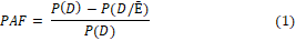
Where P(D) is the (unconditional) probability of disease over a specified time period, and P(D/Ē) is the probability of disease over the same time period conditional on non-exposed status (not exposed to the risk factor under study). The PAF is an epidemiologic measure widely used; it is the difference between overall average risk of the entire population (both exposed and unexposed people) and average risk in the unexposed, expressed as a fraction of the overall average risk [1,2].

The PAF is frequently interpreted as the proportion of disease risk or incidence that could be eliminated from the population if exposure were eliminated. The expectation is that the PAF has a practical value for those interested in public health prevention policy, particularly when dealing with an exposure that is modifiable [2]. Some authors have made a point against “relative” measures as PAF and in favour of “absolute” measures [3], an issue that has been addressed in other contexts [4].

Some of the problems around PAF are related to the concept of “causal attribution”, and to potential biases when estimating single risk factors’ PAFs under different study designs, and/or when using different counterfactuals [1,3,5-8]. However, significant limitations still exist with current strategies for estimating a PAF in multiple risk factor situations [9]; e.g. simplified approaches for PAF calculations under different study designs scenarios have been explored [10], but  discussions on new sources of potential bias that may arise, particularly the one related to the (usually made) assumption of independence (no interaction in a multiplicative model using risk ratios as effect measure [11,12], between risk factors, are limited as far as the authors know.

A few comments by Ezzati et al. [13,14] about biases when estimating multiple risk factor PAFs (reproduced below) are the main motivation of this paper.

Potential bias when assuming independence

The contribution of a risk factor to disease or mortality, relative to some alternative exposure distribution, defined as the proportional reduction in population disease or mortality that would occur if exposure to the risk factor were reduced to an alternative exposure distribution, is defined by the generalized potential impact fraction (PIF) in equation (2). The alternative (counterfactual) exposure distribution used is one that would result in the lowest population risk, referred to as the theoretical-minimum-risk exposure distribution

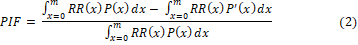
Where RR(x) is relative risk at exposure level x; P(x) is population distribution of exposure; P'(x) is alternative or counterfactual distribution of exposure; and m is the maximum exposure level.

In equation (2), RR, P, and P' can be joint relative risks and exposure distributions for multiple risk factors (i.e., x can be a vector of risk factors) [13].

To estimate the joint effects of two RFs with continuous exposure variable, each integral in the PIF relation can be replaced with

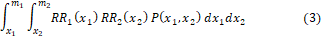
where subscripts 1 and 2 denote the two RFs and P is the joint distribution of the two exposures [13].

In equation (3) we see that independence (no interaction in a multiplicative model [11,12]) is assumed, i.e,

The paper of Ezzati et al. [13] goes on: “Because individual RRs are non-linear functions of exposure, and joint RRs the product of such nonlinear RRs, positive correlation between risk factors would usually imply a larger PAF than zero correlation (for some RRs, sub-multiplicative effect modification could result in slightly smaller PAF even with positive correlation). In turn, PAF with zero risk-factor correlation would in general be larger than negative correlation. Similarly, for categorical risk factors, positive correlation would in general result in larger PAF.”

Because these statements are relevant to assess the potential bias introduced when different unknown epidemiological scenarios are faced in practice, and corresponding assumptions are made, we consider it useful to explore in a more comprehensive manner the analytical relationships between PAF values on one hand, and functional relationships between exposure levels and RRs values, degree of correlation between RFs, and level of independence (multiplicativity [12]) between RRs, on the other hand. We have not seen works where these potential biases had been assessed in detail.

The magnitude of the biases in PAF estimations under these different scenarios, when independence is assumed, could be useful in practice because would help researchers to have an idea on the quality of PAF estimations, previous identification of which of the scenarios is closer to the actual situation they are dealing with.

Scenarios for bias assessment

For simplifying reasons, we considered just two RFs, RF1 and RF2 each with 3 equidistant exposure levels (e.g. “low”, “medium”, “high”), and also assumed the same functional relationship between exposure levels and RRs for both RFs.

Functional relationships between exposure and RRs have been modelled before [15]; in this study they are represented in terms of (global) slope (always positive) and level of concavity (up, lineal, down), as from the three equidistant exposure levels. Low slope values range from 1 to 0.27 when moving from up high to down high concavity; high slope values range from 1.5 to 0.60, also from up high to down high concavity. See table 1 for the particular combinations of slope and concavity values used. Expressions used for calculating the slope and the level of concavity are presented in the Annex.

Table 1. Functional relationship between exposure levels and RR values, in terms of first level (slope) and second level (up to down concavity) trends of RR values across equidistant exposure levels

Concavity (up to down)		Up high	Up low	Lineal	Down low	Down high
		-1.00	-0.50	0.00	0.15	0.45
slope	low	1.00	0.75	0.50	0.42	0.27
	high	1.50	1.25	1.00	0.85	0.60

Correlation (as per Spearman coefficient) between RFs was set at three categories: “positive” (0.86), “zero” (-0.03), and “negative” (-0.86).

Finally, the level of independence (no interaction in a multiplicative model, [11,12]) between RRs of RFs was set at five levels, one at the reference “100% independence”, two over-multiplicative levels, “150% independence” and “200% independence”, and two sub-multiplicative levels, “80% independence” and “60% independence”; the level of independence, IND is defined as

                             

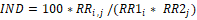
for i, j ≥ 2; i, j the levels of exposure of the RFs. RR_i,j is the combined relative risk for the  i ­­- th level of RF1 and the j ­­- th level of RF2 with respect to the combined reference level  1,1;  RR1_i is the relative risk for RF1 of the i ­­- th level of exposure with respect to the reference level 1, similarly for RR2_j and RF2. It should be noted that the assumption of independence in this multiplicative model does not necessarily mean lack of biological interaction (see e.g. [11,12]).

Several studies have assessed the combined effects of two specific RFs on particular outcomes (see some references in [14]; however, for many other situations the relevant information is not available. The scenarios considered in this work were designed as to facilitate the bias assessment when the (usual and convenient) assumption of independence is (necessarily) made, controlling for the other factors just mentioned which are easier to know as they depend not on the combined RRs but on the combined prevalence of the two RFs.

Results

The figures 1-3 present the PAF values for the three correlation levels between RFs (“positive”, “zero”, and “negative”) and the two slope levels (“low” and “high”). In each of the Figures the PAF values (vertical axis) for the 5 independence levels (different lines) and the five concavity levels (horizontal axis) are shown.

It is seen that the impact of the independence assumption on the PAF values decreases from figures 1-3; moving correlation between RF from positive to negative decreases the impact of the independence assumption (bias decreases), and moving slope levels from low to high also decreases the impact (bias decreases). Within each of the graphs it is seen that moving from high up to high down concavity (of the relationship between exposure levels and RRs values), increases the impact of the independence assumption (bias is larger when independence is assumed).

In other words, the smallest impact of the independence assumption on PAF values is observed when correlation between RFs is negative, and the functional relationship between exposure levels and RRs values has high up concavity and high slope values; the largest impact is observed when correlation between RFs is positive, and the functional relationship is characterized by a high down concavity with a low slope.

Percentage biases for the 6 scenarios in figures 1-3 are presented in tables 2-4.

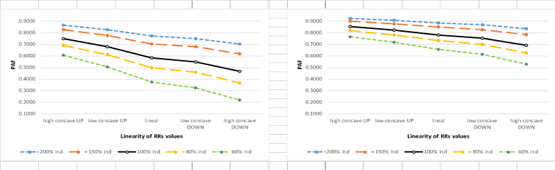
Figure 1. Relation between PAF and level of linearity of RRs, and level of independence between risk factors (A) Low slope for increasing RRs and positive correlation between RFs (B) High slope for increasing RRs and positive correlation between RFs

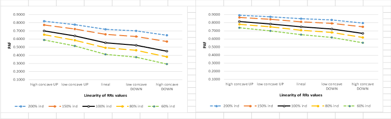
Figure 2. Relation between PAF and level of linearity of RRs, and level of independence between risk factors (A) Low slope for increasing RRs and zero correlation between RFs (B) High slope for increasing RRs and zero correlation between RFs

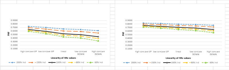
Figure 3. Relation between PAF and level of linearity of RRs, and level of independence between risk factors (A) Low slope for increasing RRs and negative correlation between RFs (B) High slope for increasing RRs and negative correlation between RFs

Table 2a. Bias (%) in PAF estimation when independence between RRs is assumed. Low slope for increasing RRs and positive correlation between RFs

Concavity	Up			Down
Independence	high	medium	none	medium	high
200%	-13.7%	-18.0%	-24.6%	-27.1%	-33.4%
150%	-9.4%	-12.5%	-17.4%	-19.4%	-24.4%
100%	0.0%	0.0%	0.0%	0.0%	0.0%
80%	7.9%	11.1%	16.7%	19.4%	27.2%
60%	23.0%	33.7%	55.8%	67.7%	111.5%

Table 2b. Bias (%) in PAF estimation when independence between RRs is assumed. High slope for increasing RRs and positive correlation between RFs

Concavity	Up			Down
Independence	high	medium	none	medium	high
200%	-7.7%	-9.4%	-11.7%	-13.4%	-17.1%
150%	-5.2%	-6.4%	-8.0%	-9.2%	-11.9%
100%	0.0%	0.0%	0.0%	0.0%	0.0%
80%	4.1%	5.1%	6.6%	7.7%	10.3%
60%	11.5%	14.5%	18.8%	22.4%	31.0%

Table 3a. Bias (%) in PAF estimation when independence between RRs is assumed. Low slope for increasing RRs and zero correlation between RFs

Concavity	Up			Down
Independence	high	medium	none	medium	high
200%	-14.6%	-18.1%	-23.1%	-25.2%	-30.4%
150%	-9.7%	-12.0%	-15.6%	-17.1%	-21.0%
100%	0.0%	0.0%	0.0%	0.0%	0.0%
80%	7.0%	9.0%	12.3%	13.8%	18.1%
60%	18.4%	23.9%	33.9%	38.7%	54.1%

Table 3b. Bias (%) in PAF estimation when independence between RRs is assumed. High slope for increasing RRs and zero correlation between RFs

Concavity	Up			Down
Independence	high	medium	none	medium	high
200%	-8.8%	-10.2%	-12.0%	-13.4%	-16.4%
150%	-5.7%	-6.7%	-7.9%	-8.8%	-10.9%
100%	0.0%	0.0%	0.0%	0.0%	0.0%
80%	4.1%	4.7%	5.7%	6.4%	8.0%
60%	10.4%	12.2%	14.6%	16.5%	21.0%

Table 4a. Bias (%) in PAF estimation when independence between RRs is assumed. Low slope for increasing RRs and negative correlation between RFs

Concavity	Up			Down
Independence	high	medium	none	medium	high
200%	-12.2%	-15.4%	-20.4%	-22.5%	-27.9%
150%	-7.3%	-9.5%	-13.0%	-14.5%	-18.6%
100%	0.0%	0.0%	0.0%	0.0%	0.0%
80%	4.1%	5.6%	8.5%	9.8%	14.0%
60%	9.3%	13.1%	20.6%	24.4%	37.2%

Table 4b. Bias (%) in PAF estimation when independence between RRs is assumed. High slope for increasing RRs and negative correlation between RFs

Concavity	Up			Down
Independence	high	medium	none	medium	high
200%	-8.3%	-9.6%	-11.3%	-12.6%	-15.4%
150%	-5.0%	-5.9%	-7.0%	-7.9%	-9.9%
100%	0.0%	0.0%	0.0%	0.0%	0.0%
80%	2.8%	3.4%	4.2%	4.9%	6.5%
60%	6.5%	7.9%	9.9%	11.6%	15.9%

Illustration

Table 5a presents correlation between RFs “alcohol consumption” (“teetotaler”, “light”, “moderate” and “heavier”) and “smoking” (“currently non-smoking” and “smoking”), and table 5b the combined relative risks of the two above RFs for type 2 diabetes [16], observed and under the independence (in a multiplicative model) assumption.

Table 5a. Correlation between Alcohol Consumption and Current Smokers in women [16]

Table 5b. Combined Relative Risks (RRs) for type 2 diabetes: observed and under independence assumption in women [16]

		RRs observed				RRs under independence assumption
		alcohol consumption				alcohol consumption
		teetotaler	light	moderate	heavier	teetotaler	light	moderate	heavier
Current smokers	no	1	0.78	0.54	0.73	1.00	0.78	0.54	0.73
	yes	1.21	1.03	0.75	0.51	1.21	0.94	0.65	0.88
For RRs of "alcohol consumption": slope=-0.105; concavity=-0.205

It is seen that the observed relative risks are close to independence, except the one corresponding to “currently smoking yes” and “alcohol consumption heavier”; the ratios of observed/expected are 109%, 115%, and 58% for cells (2,2), (2,3), and (2,4) respectively. Spearman's rank correlation coefficient between RFs is 0.129, i.e. close to zero. It is also seen that concavity is close to zero (-0.205), and global slope also close to zero (-0.105).

If we did not know the combined RRs, the observed situation based on the combined prevalence is close to scenario in figure 2a, and within this Figure close to “lineal”; according to this scenario, the percentage biases corresponding to 200%, 150%, 80% and 60% independence, when independence (100%) is assumed, would be  -23%, -16%, 12%, and 34% respectively (Table 3a).

Discussion

This study made several assumptions that limit the generalizability of its results. First, it considers only two RFs, each of them with three levels of exposure and having the same, and a simple functional relationship between these levels of exposure and the corresponding RRs in terms of slope and concavity.

It has been reported that the biases introduced from wrong assumptions when estimating PAF are in general not important (pp. 2173, [14]); however, our results show that this is not always the case.

Three levels were used for the statistical correlation between exposures of the RFs as a source of bias for the estimation of PAF, though it has been reported this does not have an important effect on the final estimation (pp.2172, [14]). From our results in Tables 2-4, correlation between exposures to RFs does seem to be non-negligible.

Sub-multiplicative models are much more frequent than over-multiplicative models [14,17] so the two levels below 100% independence (80% and 60%) should be more useful in practice than the two levels above (150% and 200%).

In summary, for simple practical situations we might find the scenarios studied in this paper useful to assess approximately the range of biases introduced when the (convenient) independence assumption is made.

Annexure

With n = number of exposure levels; x_i = 1,2,…,n; y_i = RR1, RR2,…, RRn

a) Formula for the slope: 

                                                               

b) Formula for the level of concavity:

this concavity expression provides an average of the changes in slopes for consecutive pairs of points (levels of exposure to the RF). Positive values indicate down concavity; zero values indicate a (close to) straight line, and negative values indicate up concavity.

References

1. Mansournia MA, Altman DG (2018) Population attributable fraction. BMJ 360: k757. [Crossref]
2. Levine B (2007) What does the population attributable fraction mean? Prev Chronic Dis 4: A14. [Crossref]
3. Poole C (2015) A history of the population attributable fraction and related measures. Ann Epidemiol 25: 147-154. [Crossref]
4. Seuc AH (1998) Relation between the prevalence of a characteristic and the size of the sample needed to estimate it. Eur J Epidemiol 14: 627-628.
5. Shield KD, Parkin DM, Whiteman DC, Rehm J, Viallon V, et al. (2016) Population Attributable and Preventable Fractions: Cancer Risk Factor Surveillance, and Cancer Policy Projection. Curr Epidemiol Rep 3: 201-211. [Crossref]
6. Flegal KM, Panagiotou OA, Graubard BI (2015) Estimating population attributable fractions to quantify the health burden of obesity. Ann Epidemiol 25: 201-207. [Crossref]
7. Hanley JA (2001) A heuristic approach to the formulas for population attributable fraction. J Epidemiol Community Health 55: 508-514. [Crossref]
8. Williamson DF (2010) The population attributable fraction and confounding: buyer beware. Int J Clin Pract 64: 1019-1023. [Crossref]
9. Mason CA, Tu S (2008) Partitioning the population attributable fraction for a sequential chain of effects. Epidemiol Perspect Innov 5: 5. [Crossref]
10. Bruzzi P, Green SB, Byar DP, Brinton LA, Schairer C (1985) Estimating the population attributable risk for multiple risk factors using case-control data. Am J Epidemiol 122: 904-914. [Crossref]
11. Thompson DM (2016) Evaluating biological interaction (and effect measure modification) as departures from additivity: Choosing and using additive and multiplicative models.
12. Skrondal A (2003) Interaction as departure from additivity in case-control studies: a cautionary note. Am J Epidemiol 158: 251-258. [Crossref]
13. Ezzati M, Hoorn SV, Rodgers A, Lopez AD, Mathers CD, et al. (2003) Estimates of global and regional potential health gains from reducing multiple major risk factors. Lancet 362: 271-280. [Crossref]
14. Ezzati M, Lopez AD, Rodgers AA, Murray CJL (2004) Comparative Quantification of Health Risks: The Global and Regional Burden of Disease Attributable to Selected Major Risk Factors. Geneva: WHO.
15. Traskin M, Wang W, Ten Have TR, Small DS (2013) Efficient estimation of the attributable fraction when there are monotonicity constraints and interactions. Biostatistics 14: 173–188.
16. Joosten MM, Grobbee DE, van der A DL, Verschuren WM, Hendriks HF, et al. (2010) Combined effect of alcohol consumption and lifestyle behaviors on risk of type 2 diabetes. Am J Clin Nutr 91: 1777-1783. [Crossref]
17. Begg CB (2001) The search for cancer risk factors: when can we stop looking? Am J Public Health 91: 360-364. [Crossref]