Various high-percentage high-incidence medical conditions, acute or chronic, start at a particular age of onset t1 [yrs.], accumulate or progress rapidly, with a system time constant t0 [yrs.], typically from one week to five years, and then level off at a saturation plateau level <S>, ultimately affecting ten to ninety-five percent of the population. This report investigates the prevalence and incidence functions for myopia and high myopia as a function of age. This is a retrospective study. Fundamental prevalence vs. time and incidence vs. time results allow continuous prediction of myopia and high myopia population fractions as a function of age. Nine reports are calculated with N = 444,600 subjects, from S. E. Asia. No interventions other than usual regular eye exams, and subsequent indicated refraction change. The main result is continuous prediction of myopia prevalence-time data along with incidence rate data [% / year], age of onset [years], system plateau level, and system time constant [yrs.]. These parameters apply to progressive myopia and high myopia ( R < - 6 D ), useful over several decades. The primary finding of this research is that the prevalence ratio of high-myopes (R < -6.0 D) to common-myopes is expected to increase from 25% entering college, to 50% or more after college. These statistics are particularly relevant to the many years of study required by M.D., Ph.D., and M.D. / Ph.D. programs.
prevalence, incidence, myopia, high myopia, exponential equations, reading glasses, time constant, onset age, saturation level
Pr(t) = myopia prevalence fraction as a function of time [ % ]
In(t) = myopia incidence rate as a function of time [ % / year ]
t0 = myopia time constant [years]
t1 = myopia onset age [years]
t2 = onset age [years] for advanced myopia
<S> = saturation plateau level [%], 30% - 95% for myopia
95% CI = 95% conf. interval, r = correl. coefficient
<std.err.> = r.m.s. error @ regression line, typically +/- 2%
The myopia prevalence fraction Pr(t) [ % ] versus time and the myopia incidence rate In(t) [ %/yr ] versus time are fundamental mathematically coupled functions, basic to the understanding of progressive myopia [1-5].
In general, medical conditions may be communicable or non-contagious, endemic or epidemic, inherited or acquired. The incidence rate function In(t) [%/yr.] is often mis-understood - for myopia, a typical incidence rate of 16% percent per year, means one can expect sixteen new myopes each year, from each class of one-hundred students, at that age bracket. Practical ophthalmic examples of prevalence and incidence equations include retinopathy of prematurity ( R.O.P.), juvenile onset myopia, with onset age ranging from t1 = 0 to 12 yrs., adult onset glaucoma [6] with onset age t1 = 30 years, macular degeneration, cataract development, and presbyopia, with onset around age 40.
Population demographic and epidemiologic surveys often include prevalence measurements, but not incidence data, incidence but not prevalence data, or prevalence without age-specific data. A system time constant t0 [yrs.] is rarely cited. In this report, we relate these fundamental parameters with basic equations, as applied to the progression of myopia, of epidemic proportions in some populations [3,7]. Some reports simultaneously include prevalence and incidence rates, at age-specific time intervals, allowing for an improved understanding of the problem of myopia [3,4,7-20].
Usually, incidence data In(t) [ %/yr ] and prevalence Pr(t) [%] are not available simultaneously. Similar equations for prevalence as a function of time or age Pr(t) are derived by Brinks & Landwehr (2013, 2015). Basic exponential equations for prevalence Pr(t) and incidence In(t) yield four key system parameters: onset age t1 [yr], time constant t0 [yr], saturation plateau level <S> [%] , and initial incidence rate In(t1) [%/yr]. These then, in turn, allow direct comparisons between one data set and another, both cross-sectional and longitudinal.
Basic equations: Myopia prevalence as a function of time is modeled with the following exponential equation [4]:
Pr(t) = 0.90 [ 1 - exp(-(t-t1)/t0) ] (1)
The derivative d [ Pr ( t ) ] / dt is given by
In(t) = 0.90 [ (1/t0) exp(-(t-t1)/t0) ] (2)
where t0 [yrs.] is the system time constant, t1 [yrs.] is the onset age, and <S> = 0.90 is the saturation plateau level. For myopia, the saturation plateau level <S> = 0.90 indicates that by age 25 to 30 years old, 90% percent of these populations will develop myopia. The general format for the exponential prevalence equation, with saturation plateau <S> is:
Pr(t) = <S> [ 1 – exp ( -(t-t1) / t0 ) ] (2a)
As derived in Theoretical Results below, Eqs. 4 & 5. Data are from the studies of Goh & Lam [11], Lin et al. [14,15], Saw et al. [4], Fan et al. [1,8], Greene [9], Tay et al. [17], Lam & Goh [13], Greene et al. [2].
Statistics: Least squares regression calculates an average incidence rate In(t) = 4.7 % per year. Confidence limits on the incidence rate are In = [ 95% CI: 2.1 to 7.3 %/yr ] (Figure 1). This means one can expect 2.1 to 7.3 new cases of myopia per year, on average, from each class of 100 at the same education level, Figures 2 and 3. The exponential equations predict much higher initial incidence rates In(t1), i.e. 15% to 20% per year, consistent with the incidence rate data, as shown in Figures 2 and 3. Table 1 displays the exponential prevalence function Pr(t) and incidence function In(t). The myopia prevalence vs. time function Pr(t) [yrs] and myopia incidence vs. time function In(t) [%/yr] are continuously generated and compared with student data, Figures 1 and 2.
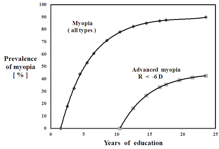
Figure 1. The myopia prevalence function Pr(t) [%] vs. years of education, N=9 studies, [4]. Pr(t) = 0.90 *[ 1 – exp ( - ( t – t1 ) / to ) ], to = 4.5 yrs. , t1 = 1.5 yrs. For the advanced myopes, Pr(t) = <S> [ 1 – exp ( - ( t – t2 ) / to )], where to = 4.5, t2 = 9 , S=0.45.
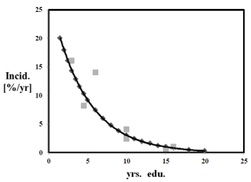
Figure 2. Myopia incidence function In(t) [%/yr.] i.e. # of new cases per year, per class of 100, N = 7 studies. In(t) = 0.90 [ (1/to) exp(-(t-t1)/to) ] +/-2.6%/yr., to = 4.5 yrs., t1 = 1.5 yrs., [2]. For advanced myopia, In(t) = <S> * [ ( 1 / to ) * exp ( - ( t – t2 ) / to ) ].
Table 1. Prevalence and incidence functions vs. time ( t0 = 4.5 yrs., t1 = 1.5 yrs).
|
t [yrs.]
|
Pr(t) [%] (*)
|
In(t) [%/yr] (**)
|
|
1.5
|
0.0
|
17.9
|
|
2.5
|
17.9
|
14.4
|
|
3.5
|
32.3
|
11.5
|
|
4.4
|
43.8
|
9.2
|
|
5.5
|
53.0
|
7.4
|
|
6.5
|
60.4
|
5.9
|
|
7.5
|
66.3
|
4.7
|
|
8.5
|
71.0
|
3.8
|
|
9.5
|
74.8
|
3.0
|
|
10.5
|
77.8
|
2.4
|
|
11.5
|
80.2
|
2.0
|
|
12.5
|
82.2
|
1.6
|
|
13.5
|
83.7
|
1.3
|
|
14.5
|
85.0
|
1.0
|
|
15.5
|
86.0
|
0.8
|
|
16.5
|
86.8
|
0.6
|
|
17.5
|
87.4
|
0.5
|
(*) Pr(t) = prevalence vs. time function
(**) In(t) = Incidence vs. time function
Theoretical results: Myopia incidence rates [%/yr] are 5 to 10 times more rapid, during the juvenile and teen years, compared to the college and university years. Figure 1 presents prevalence as a function of years of education Pr(t), using the data from [10], and theory from Eq. (1). Figure 2 shows incidence as a function of time In(t), using data from [10], and theory from Eq. (2).
For comparison with the exponential model, Figure 3 displays least squares regression statistics, yielding the following:
prev(t) = 0.047(t) + 0.178 (x 100 %) (3)
where t = years of education, correlation r = 0.88, N=9, <std.err.> = +/-10.6% about regression line, constant incidence rate < In > = 4.7 % per year, [95% CI: 2.1 to 7.3 %/yr].
Eq. (1) and (2) are derived setting the number of new incident subjects proportional to the residual fraction of normal subjects, yielding :
In ( t ) = k x [ 1 - Pr( t ) ] (4)
From this, the inverse relation between incidence and time constant also can be derived:
In ( t1 ) = < S > / t0 (5)
An important sub-group, accounting ultimately for ½ the total, the advanced myopes are presented in Figure 1, showing the myopia prevalence function Pr(t) [%] vs. years of education, Pr(t) = 0.90 *[ 1 – exp ( - ( t – t1 ) / to ) ], to = 4.5 yrs. , t1 = 1.5 yrs. For the advanced myopes, Pr(t) = <S> [ 1 – exp ( - ( t – t2 ) / to ) ], where to = 4.5, t2 = 9 , S = 0.45. Table I presents the results of Eqs. (1) and (2), including myopia prevalence fraction [%] and incidence rate [%/yr] .
Applications: Basic exponential equations presented here can continuously predict the prevalence Pr(t) [%] and incidence rate In(t) [%/yr] functions for myopia development. Symmetrically, the incidence function is derived from the prevalence function, the prevalence is the integral of the incidence. Thus, these are coupled equations. The initial incidence rate is inversely related to the system time constant, Eq. 5. For instance, an initial incidence In(t1) = 33 new cases per year, per 100, implies a time constant t0 = 3 yrs. for a plateau level of <S> = 1. For the analysis of myopia development, the time constant is t0 = 4.5 years, which is comparable to the individual myopia time constant 3 < t0 < 5 years, as reported by Medina & Fariza [12].
Least squares regression, while useful for prevalence data, Eq. 3 and Figure 3, considerably underestimates the incidence rate. Nevertheless, this approximation is reasonable, at a constant incidence level <In> = 4.7 %/yr. [95%CI: 2.1 to 7.3 %/yr.]. By comparison, the exponential equations are quite accurate, able to predict the incidence rate data within +/-2.6 %/yr, over the entire age range, Figure 2.
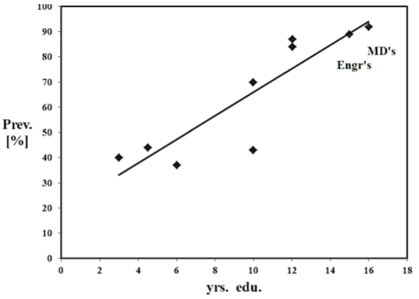
Figure 3. Linear regression of myopia prevalence as a function of years of education, N=9 demographic studies. Pre-medical N=345 students, H.K., engineers N=39 students, U.S. On average, myopia incidence = 4.7 %/yr., conf. limits [95%CI: 2.1 to 7.3 %/yr.], [2].
Pan, Ramamurthy & Saw [3] present a summary of N=12 worldwide age-specific prevalence studies, examining juvenile myopia from China, India, Malaysia, Nepal, United States, South Africa, and Chile. More recent prevalence studies include Kim et al. [12], and Sun et al. [16], who report myopia prevalence Pr = 95.5%, N=5083, for college students, and Yip et al. [18], and Lee et al. [5] who report 83.3% myopia prevalence, N=2805, among university students.
In this report we investigate the two simplest mathematical models available for prevalence and incidence, linear regression and exponential regression. Each may be applied to ophthalmic prevalence and incidence studies, allowing modeling of progressive myopia, glaucoma, presbyopia, and cataract, each with a specific onset age range and system time constant. These equations are accurate over the course of 2 to 3 decades.
For myopia, onset age, time constant, and saturation plateau level are fundamental system parameters derived from age specific prevalence data. In turn, these characteristic system parameters may be compared with the results of future myopia intervention studies.
High Myopia: Ordinary uncomplicated myopia (R > -6 D) is quite common, not considered a disease, per se. However, high myopia ( R < -6 D ) can result in some serious problems, that may lead to detrimental ramifications, involving the retina, choroid, sclera, vitreous and lens. The prevalence fraction Pr(t) [%] and incidence rates In(t) [%/year] of high myopia are therefore important to examine separately. Mathematically, the high myopia prevalence fraction is a matter of a delayed onset t2 of 9 - 12 years after t1, and a reduced saturation plateau level 50%, Greene & Medina [21], Eq. (6) graphed in Figure 1
Pr(t) = <S> * [ 1 - exp ( - ( t - t2 ) / t0 ) ] (6)
The literature has many mathematical models of prevalence for various types of contagious or acquired diseases [5,6,17,18,22-27], some requiring multiply linked differential equations (i.e. SEIR = susceptible, exposed, infected, and resistant population fractions), including linear and exponential models, compared here, power law, binomial, quadratic, Markov, random, and oscillating (Podgor & Leske [26], Keiding [27]). For progressive myopia, the variables of interest, in addition to time, include age, discussed here, ethnicity, location, discussed here, inherited factors, and the near-point environment.
The primary finding of the research presented here is that the prevalence ratio of high-myopes (R < -6.0 D) to common-myopes is expected to increase from 25% entering college, to 50% or more after college, Figure 1. These statistics are particularly relevant to the many years of study required by M.D., Ph.D., and M.D./Ph.D. programs.
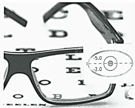
Figures 4 and 5 below schematically show the -3.0 to -4.0 diopter demand on the eye’s focusing system caused by studying, typical of some college students, and the proposed optical solution to this problem, by counter-acting the -3.0 D near-point environment with a compensating +3.0 D (+) lens.

Figure 5. Reading glasses for a -5.00 D. college myope. (+) Add technology is used by both bifocals and progressive addition lenses, “PAL’s”. PAL’s are “no-line” bifocals. Basically, these (+) Add reading glasses are distance compensators, with a +3.00 D Add for reading.
The authors thank Frank Young, Otis Brown, Antonio Medina, and Bill Baldwin for many helpful discussions.
The authors have no proprietary or financial conflicts of interest.
- Fan DS, Lam DS, Lam RF, Lau JT, Chong KS, et al. (2004) Prevalence, incidence, and progression of myopia of school children in Hong Kong. Invest Ophthalmol Vis Sci 45: 1071-1075. [Crossref]
- Greene PR, Vigneau ES, Greene J (2015) Exponential prevalence and incidence equations for myopia. Clin Exp Optom 98: 210-213. [Crossref]
- Lam CS, Goh WS (1991) The Incidence of Refractive Errors Among School Children in Hong Kong in Relationship with the Optical Components. Clin Exp Opt 74: 97-103.
- Lin LL, Shih YF, Hsiao CK, Chen CJ (2004) Prevalence of myopia in Taiwanese schoolchildren: 1983 to 2000. Ann Acad Med Singapore 33: 27-33. [Crossref]
- Pan CW, Ramamurthy D, Saw SM (2012) Worldwide prevalence and risk factors for myopia. Ophthalmic Physiol Opt 32: 3-16. [Crossref]
- Sun J, Zhou J, Zhao P, Lian J, Zhu H, et al. (2012) High prevalence of myopia and high myopia in 5060 Chinese university students in Shanghai. Invest Ophthalmol Vis Sci 53: 7504-7509. [Crossref]
- Dolgin E (2015) The myopia boom. Nature 519: 276-278. [Crossref]
- Fan DS, Cheung EY, Lai RY, Kwok AK, Lam DS (2004) Myopia progression among preschool Chinese children in Hong Kong. Ann Acad Med Singapore 33: 39-43. [Crossref]
- Greene PR (1986) Gaussian and Poisson blink statistics: a preliminary study. IEEE Trans Biomed Eng 33: 359-361. [Crossref]
- Greene PR, Medina A (2016) Analogue Computer Model of Progressive Myopia – Refraction Stability Response to Reading Glasses. J Comput Sci Syst Biol 9: 104.
- Medina A, Fariza E (1993) Emmetropization as a first-order feedback system. Vision Res 33: 21-26. [Crossref]
- Medina A (2015) The progression of corrected myopia. Graefes Arch Clin Exp Ophthalmol 253: 1273-1277. [Crossref]
- Medina A (2016) Detecting the effect of under-correcting myopia. Graefes Arch Clin Exp Ophthalmol 254: 409-410. [Crossref]
- Goh WS, Lam CS (1994) Changes in refractive trends and optical components of Hong Kong Chinese aged 19-39 years. Ophthalmic Physiol Opt 14: 378-382. [Crossref]
- Lin LL, Shih YF, Lee YC, Hung PT, Hou PK (1996) Changes in ocular refraction and its components among medical students--a 5-year longitudinal study.” Optom Vis Sci 73: 495-498.
- Brinks R, Landwehr S, Icks A, Koch M, Giani G (2013) Deriving age-specific incidence from prevalence with an ordinary differential equation. Stat Med 32: 2070-2078. [Crossref]
- Brinks R, Landwehr S2 (2015) A new relation between prevalence and incidence of a chronic disease. Math Med Biol 32: 425-435. [Crossref]
- Greene PR, Grill ZW, Medina A (2016) Mathematical Models of College Myopia. Optik (Stuttg) 127: 896-899. [Crossref]
- Kim MH, Zhao D, Kim W, Lim DH, Song YM, et al. (2013) Heritability of myopia and ocular biometrics in Koreans: the healthy twin study. Invest Ophthalmol Vis Sci 54: 3644-3649. [Crossref]
- Saw SM, Tong L, Chua WH, Chia KS, Koh D, et al. (2005) Incidence and progression of myopia in Singaporean school children. Invest Ophthalmol Vis Sci 46: 51-57. [Crossref]
- Greene PR, Medina A (2016) Refraction data survey: 2nd generation correlation of myopia. Int Ophthalmol 36: 609-614. [Crossref]
- Tay MT, Au Eong KG, Ng CY, Lim MK (1992) Myopia and educational attainment in 421,116 young Singaporean males. Ann Acad Med Singapore 21: 785-791. [Crossref]
- Lee JH, Jee D, Kwon JW, Lee WK (2013) Prevalence and risk factors for myopia in a rural Korean population. Invest Ophthalmol Vis Sci 54: 5466-5471. [Crossref]
- Yip VC, Pan CW, Lin XY, Lee YS, Gazzard G, et al. (2012) The relationship between growth spurts and myopia in Singapore children. Invest Ophthalmol Vis Sci 53: 7961-7966. [Crossref]
- Quigley HA, Vitale S (1997) Models of open-angle glaucoma prevalence and incidence in the United States. Invest Ophthalmol Vis Sci 38: 83-91. [Crossref]
- Podgor MJ, Leske MC (1986) Estimating incidence from age-specific prevalence for irreversible diseases with differential mortality. Stat Med 5: 573-578. [Crossref]
- Keiding N (1991) Age-Specific Incidence and Prevalence: a Statistical Perspective. J Roy Statist Soc A 154: 371-412.